C Pop quiz answers
C.1 Chapter 1. Reading a value stream map
The answers for the Pop Quiz will appear shortly (after the seminar).
Table 1.4 asked the following questions that can be answered by inspecting Figure 1.1.
- What is the pacemaker process? The assembly stage
- How long is the planning cycle? One week
- What level of availability is achieved by the vendor managed inventory? 88.46%
- What is the variance of the demand process? 29
- How much raw material inventory do we hold on the average? 36.5
- What is the safety stock level at the raw material inventory location? 30
- What is the variance of the confirmed production plan? 123.6
- What is the variance of the vendor managed inventory? 199.4
- What is the suppliers fill rate? 96.48
- What forecasting method is used in the ERP system? Exponential smoothing, with a smoothing parameter of \(\alpha=0.4\)
- What is the customers lead time? \(T_p=2\)
- How far away is the supplier? 200km
- How bullwhip is generated by the planning system? The system bullwhip is 3.97
- What is the confirmed (planned) bullwhip? The planned bullwhip is 4.26
- What is the supplier’s bullwhip? The supplier’s bullwhip is 11.74
- What is the suppliers NSAmp? The suppliers NSAmp = 728 / 123.6 = 5.88
- What is maximum customers demand? This information is not given on the VSM
- What is the maximum quantity assembled? 44
- What replenishment strategy is used in the production planning system? Order-up-to (OUT) policy
- Detailed scheduling is conducted with the aid of which planning tool? Gantt charts
C.2 Chapter 2. Selecting your replenishment strategy
Table 2.2 presented some Yes or No type questions that should lead you to your replenishment strategy. Each product/customer location pairing in your portfolio may have a different answer to the 18 questions, but Table C.1 should give you some ideas of suitable strategies.
| Question | Yes | No |
|---|---|---|
| Q1 | OUT | Level, POUT |
| Q2 | POUT | OUT, Pure pull |
| Q3 | Level, POUT | OUT, Pure pull |
| Q4 | Batch | Anything but Batch |
| Q5 | Level, POUT | OUT, Pure Pull, Batch |
| Q6 | OUT | POUT |
| Q7 | Level, POUT | OUT |
| Q8 | Level, POUT | OUT |
| Q9 | OUT | POUT |
| Q10 | POUT | Any strategy |
| Q11 | POUT | Level |
| Q12 | POUT | Any strategy |
| Q13 | POUT, OUT | Any strategy |
| Q14 | POUT | Pure Pull, Level, OUT |
| Q15 | OUT | POUT |
| Q16 | POUT | Any strategy |
| Q17 | OUT, POUT | Batch |
| Q18 | Forecast | Any strategy |
C.3 Chapter 3. Selecting a forecasting mechanism
Note, the answers to this pop quiz change depending on the supply chain setting, the costs, the objectives, and the replenishment strategy. It is a qualitative choice and you could have other equally valid, but different, answers.
| Question | Answer | Comments |
|---|---|---|
| Q1 | Damped Trend | Convex increasing demand, use \(\phi>1\). |
| Q2 | Exponential Smoothing, Moving Average or Naïve | A zero forecast or a forecast based on Croston’s Method could also have been used (but both are not explained in this workbook). |
| Q3 | Exponential Smoothing or Moving Average | Small fluctuations around a constant, un-trended mean. |
| Q4 | Holts | Linearly increasing demand. Damped trend with \(\phi=1\) could also have been used. |
| Q5 | Exponential Smoothing, Moving Average | Two non-trended time series, with a step change between them. Use small \(\alpha\) or \(n\) during the period of change if its timing is known. |
| Q6 | Holt’s | Linearly increasing demand. Damped trend with \(\phi=1\) could also have been used. |
| Q7 | Damped Trend | The time series is concave increasing in the first half, use \(0<\phi<1\). In the second half, the time series is concave decreasing, use \(\phi>1\). |
| Q8 | Damped Trend | The time series is concave decreasing, use \(\phi>1\). |
| Q9 | Damped Trend | The time series is convex decreasing, use \(1>\phi>0\). |
| Q10 | Exponential Smoothing or Moving Average | Two step changes between un-trended demand. Use small \(\alpha\) or \(n\) during the period of step change if its timing is known. |
| Q11 | Exponential Smoothing or Moving Average | Small fluctuations around a constant, un-trended (albeit small) mean. |
| Q12 | Damped Trend or Holt’s | The first quarter of the time series is convex increasing, use \(\phi>1\). The second quarter is concave increasing, use \(1>\phi>0\). The third quarter is concave decreasing, use \(\phi>1\). The final quarter is convex decreasing, use \(1>\phi>0\). |
C.4 Chapter 4. Setting the cadence of your pacemaker

Figure C.1: This section is currently under construction
C.5 Chapter 5. The shortest path through the product wheel
Figure C.2 shows that the answer to the shortest path through the product wheel is \(\{A,B,D,C,A\}\) and the minimised cost is 14. Figure C.2(a) translates the cost matrix in Table 5.2 into a direct acyclic graph. Figure C.2(b) provides the workings of the solution.
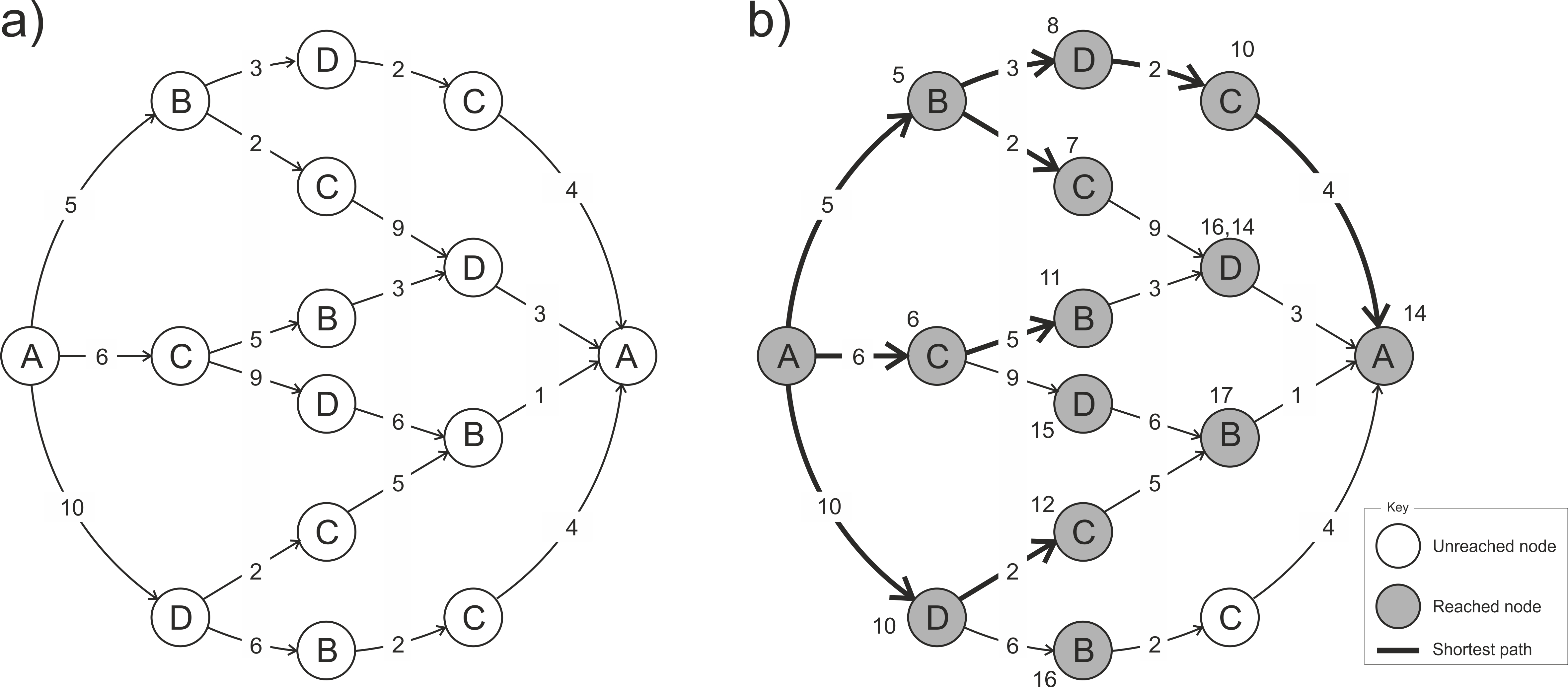
Figure C.2: Solution to the product wheel pop quiz