Chapter 3 Forecasting: Throwing your inventory javelin over the lead-time
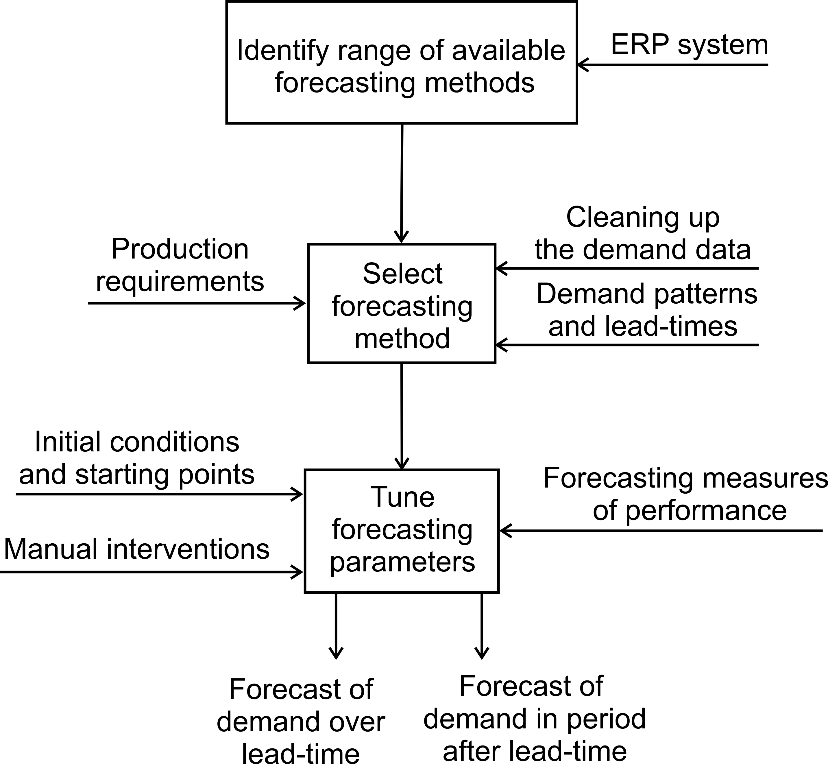
Having decided upon your replenishment strategy the next task is to forecast demand. All replenishment strategies require forecasts of some form or another. If you are pursuing the Pure Pull strategy, you will need to provide some future guidance of the likely demand so that you and your supplier can plan capacity requirements, hire staff, and order raw materials for example. Forecasts provide future guidance. If you are using a Batch strategy, then you will need an estimate of the demand rate to determine the batch size. If you are using the OUT/POUT policy two forecasts are required: one of demand over the lead-time, and another of the demand in the period after the lead-time. If you have adopted a Forecast only replenishment strategy, you will need to create a forecast as that is all there is to the strategy.
Inventory requirements are related to forecasting accuracy. If we could precisely predict customer demand in the period after the lead-time and review period, we could set up our production and distribution system to place the product in the customer’s hands at the precise moment it is desired. In this scenario, we do not need any inventory to satisfy demand, see Figure 3.1. Inventory is required in MTS situations because we cannot precisely predict what the customer will need in the future. Inventory requirements are directly proportional to the standard deviation of the forecast error over the production (and supplier) lead-time.
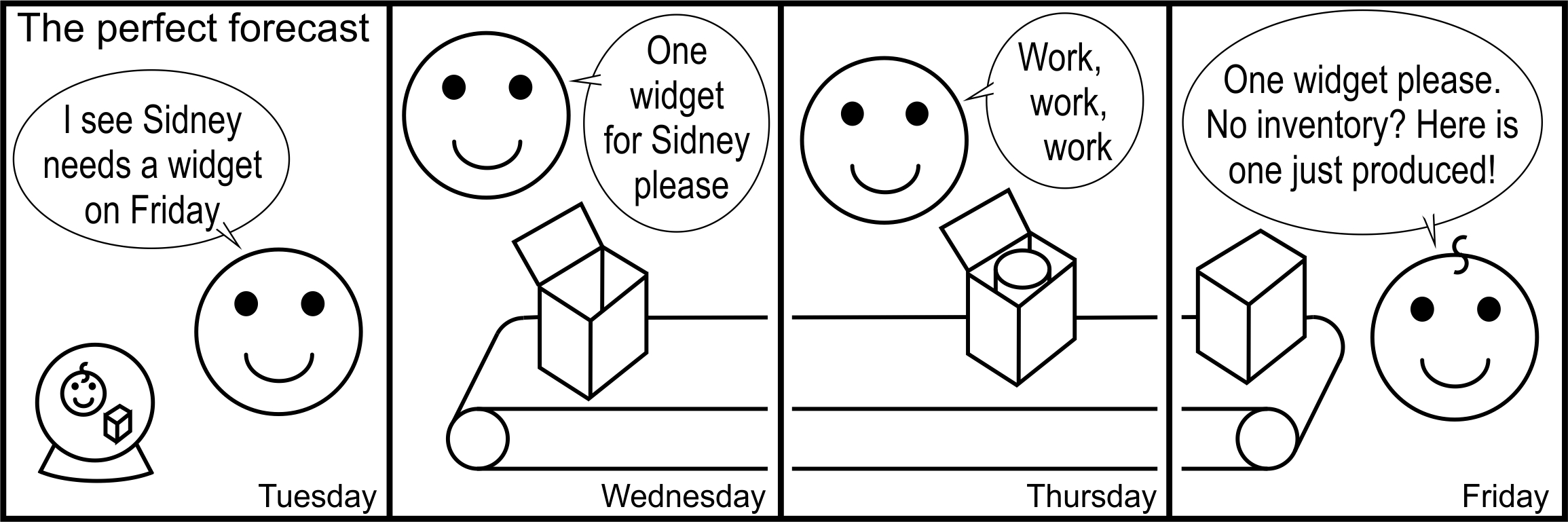
Figure 3.1: The perfect forecast
As it is harder to predict further into the future, there are many positive benefits to reducing lead-times: forecasts are more straightforward to generate and more accurate in the near term, inventory requirements are reduced, and less Bullwhip is created. However, even with zero physical lead-time, we still need to forecast one-period-ahead due to the sequence of events in periodic replenishment policies. Plus, your supplier will expect some guidance on future requirements so that he may plan for his future, see Chapter 6. Generating appropriate forecasts is, therefore, an essential activity.
Given the importance of forecasts for supply chains, this Chapter considers the following topics: the use and utility of forecasts, the demand, different forecasting methods, measures of forecast performance, tuning forecast parameters, and manual adjustments/interventions.
3.1 Specifying forecasts for your value stream
Often we do not know what is going to happen in the future. However, knowing what the future holds can lead to better business decisions. Perfectly predicting the future is impossible, but a reasonable estimate is better than complete ignorance. Thus, there is a need to forecast. Some companies like to advocate a single forecast for the whole company, but they use forecasts for many different purposes.
Typical forecasting applications
- Establishing sales goals.
- Budget planning.
- Staff hires.
- Capacity acquisitions.
- Planning promotions.
- Anticipating warranty returns.
- Communicating business performance to Wall Street.
- Ordering raw materials from suppliers.
- Setting production and distribution targets.
It is easy to appreciate that the forecasting objective in each of these contexts is different, and often incompatible, with the needs of production and distribution planning. If a company forecast is present, it should be evaluated against the requirements of the production and distribution system. If your company forecast is easily out-performed by other (perhaps algorithmic) forecasts, then maybe the company forecast should be ignored. Instead, a prediction based on real demand data should be generated accounting for the specific needs of the production and distribution departments.
3.2 What is demand?
Before we create a forecast, we first take a look at what we are trying to forecast, demand. What is demand? The obvious answer is that it is the sales to the customer. However, the situation is often more complicated than this. Sometimes the consumer desires the product, but there is no inventory. In this case, the sale cannot occur, and the actual demand cannot be observed. In some instances, unsatisfied demand is backlogged. That is, the demand is saved for the future–it is backlogged–and when inventory does become available, it is shipped to the customer. In other cases, the unsatisfied demand results in a lost sale. Lost sales occur when the customer either decides to: not buy any product, purchase a substitute product, or diverts his demand to a competitor. A backlog is easier to identify than a lost sale, but in many situations, companies have no idea of either of these two quantities.
Many companies do not simply sell their product to anybody. To be able to purchase products, you may require a line of credit with the supplier. Usually, customers value this credit–they can receive product now and pay for it later. However, credit is allocated by the ability to pay and historical performance of paying on time. Financially secure companies, with a long history of prompt payment, may receive a high credit rating and be allowed to place large orders. However, customers in financial trouble, or those with a history of not paying promptly, may be supplied with only small amounts of the product until they are paid for, or not supplied at all. In such a case, we say that demand is lost due to a credit hold.
In some cases, demand may be contaminated by shrinkage (damage, decay, evaporation, theft by customers or staff), or there may be issues with product going out-of-date or otherwise deteriorating. In other cases demand may be lost, not because it is out-of-stock, but because the product is not where it should be (it is misplaced–perhaps the inventory is in an unloading bay or in the back room) and the customer can’t find, or does not have access to, the product. In some industries, customer returns are allowed that may result in negative demand.
Another factor is the quantification of demand. Are single units of product sold (cars for example)? Or boxes/crates of items (boxes of beer)? Or is the product sold by volume or weight (liquids, powders, granules)? Or is the demand so high that rounding issues can be ignored?
Notwithstanding all of the above issues, demand may still be hard to determine consistently across all of your customers. For example, in a VMI setting, the demand signal may be represented by an ERP transaction that is triggered when your inventory was removed from your customer’s stores to be used on his production line. Or the demand signal could represent claimed inventory that is back-flushed through the bill of materials (BOM) by your customer’s ERP system as a completed product exits your customer’s production line. In the former case the VMI inventory, or part of the VMI inventory, may be placed back into the stores if the whole batch is not required. This movement to the stores can result in negative demand if returned in a later period without sufficient demand. In the latter case, back-flushed demand can only be observed after the production lead-time which may be several periods in duration. There may also be problems with achieving a proper and consistent account of scrap, yield loss, and/or quality, especially as all these reasons need to be properly coded in ERP systems; does everyone, in all of your supply chain know this and consistently do it correctly?
As you may be selling to many different customers, on different trading terms, with different IT systems, it is likely that a consistent interpretation of demand is not present. You should investigate what the demand represents and take steps to get a clean, consistent set of data. This will include making sure that all parts of your value stream, and your customer’s value system, correctly execute their required transactions promptly. For example, when a container arrives, is it emptied and all items booked into raw materials/goods in immediately? Are quality holds and scrap recorded consistently in a timely fashion everywhere in your supply chain?
Do not underestimate the scale of this task. In a global supply chain, you will have a global training problem where business practices and processes need to be aligned. Company records will need to be checked, corrected, and cleaned. Accurate, consistent and timely data is essential for proper supply chain control. In some cases, records may be locked, and efforts have to be made to find the owner of the lock and release the data for modification.
3.3 Common forecasting methods
There are many different forecasting techniques available. Practically it will be best to first look at your ERP system7 to see which methods are available to use without having to write code. To give you a flavour of how different forecasting methods work we will consider five common forecasting methods, see Table 3.1.
| Forecasting method | Characteristic equation | Forecasting parameters | Use when |
|---|---|---|---|
| Naïve | \(\hat{d}_{t+n|t}=d_t\) | None | Demand has no natural mean and demand is non-stationary or when a Pure Pull strategy is present. |
| Moving average | \(\hat{d}_{t+n|t}=\frac{\sum^{m-1}_{t=0} d_{t-i}}{m}=\frac{d_t+d_{t-1}+...+d_{t-(m-1)}}{m}\) | \(m\) | Extreme smoothing is required; use an average of all previous demand (set \(m\) as large as possible). |
| Exponential smoothing | \(\hat{d}_{t+n|t}=\hat{d}_{t+n-1|t-1}+\alpha (d_t-\hat{d}_{t+n-1|t-1})\) | \(\alpha\) | Demand has no natural mean and demand is non-stationary or when normally stable demand is likely to experience a step change in its level. |
| Holt’s method | \(\hat{a}_t=(1-\alpha)(\hat{a}_{t-1}+\hat{b}_{t-1})+\alpha d_t,\) \(\hat{b}_t=\hat{b}_{t-1}(1-\beta)+\beta(\hat{a}_t-\hat{a}_{t-1}),\) \(\hat{d}_{t+n|t}=\hat{a}_t+n\hat{b}_t.\) | \(\alpha, \beta\) | Demand has an increasing or decreasing linear trend over the lead-time and review period. |
| Damped trend | \(\hat{a}_t=(1-\alpha)(\hat{a}_{t-1}+\phi \hat{b}_{t-1})+\alpha d_t,\) \(\hat{b}_t=\phi \hat{b}_{t-1}(1-\beta)+\beta(\hat{a}_t-\hat{a}_{t-1}),\) \(\hat{d}_{t+n|t}=\hat{a}_t+\big(\sum^n_{i=1} \phi^ i \big) \hat{b}_t =\hat{a}_t+\frac{\phi(\phi^n-1)}{\phi-1} \hat{b}_t.\) | \(\alpha, \beta, \phi\) | Demand has an exponential growth or exponential decay over the lead-time and review period. |
These five methods have been selected as they provide reasonably robust solutions to the most likely encountered practical situations. Before we consider the forecasting methods in detail, we will first define some notation and the sequence of events in a forecasting system.
Notation. In all cases, \(d_t\), is the demand at time \(t\). The time index \(t\) is an integer (think of it as a week number) that tells us which period the demand occurred in. We assume the current and all previous demand is known and is the input into the forecasting system. The output of the forecasting system is a set of forecasts of demand in future periods, \(\hat{d}_{t+n|t}\). Here the hat on the \(d\), tells us that it is a forecast of demand, \(d\). The first subscript, \(t+n\), tells us this is a forecast of demand in period \(t+n\), where \(n\) is a positive integer. The second subscript, \(t\), informs us the forecast was made at time \(t\) (and uses only the information available at time \(t\)).
The sequence of events in forecasting systems. Figure 3.2 illustrates the sequence of events in a typical forecasting/ERP system and highlights that the forecast, \(\hat{d}_{t+1|t}\), is made at the end of the period. It uses data from the current period \(t\) and all previous periods, implying that the forecast \(\hat{d}_{t+1|t}\) is a forecast of the demand in period \(t+1\).
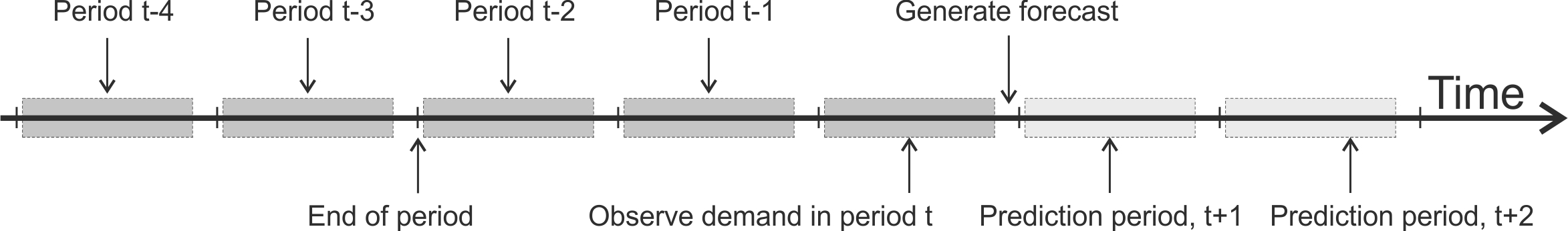
Figure 3.2: The sequence of events commonly assumed in forecasting applications
3.4 Review of common forecasting methods
Table 3.1 highlighted five different forecasting methods that we will review in this Chapter. While this list is not exhaustive, it does allow us to consider a wide range of the issues involved in forecasting.8 We will now review each method.
3.4.1 Naïve forecasting
The naïve forecasting method is the simplest forecasting method which sets all future forecasts equal to the current demand. Naïve forecasts may be appropriate when demand is so unpredictable that there is no reason to believe that previous demand has any influence on future demand. The naïve forecasting method has no parameters to set, requires no previous demand data points to be kept or stored, and all future forecasts are equal to each other. Table 3.2 details how the naïve demand forecast is calculated. Also, notice that there are no initial conditions (start-up period) required with this forecasting mechanism. As the forecast is the same as the demand, the forecast variability is also the same as the demand variability and a large amount of Mura and Muri can be generated when naïve forecasts are used inside the OUT replenishment policy.
| Time, \(t\) | Demand, \(d_t\) | Forecast of all future demand, \(\hat{d}_{t+n|t}=d_t\) |
|---|---|---|
| \(1\) | \(d_1=10\) | \(\hat{d}_{1+n|1}=d_1=10\) |
| \(2\) | \(d_2=6\) | \(\hat{d}_{2+n|2}=d_2=6\) |
| \(3\) | \(d_3=8\) | \(\hat{d}_{3+n|3}=d_3=8\) |
| \(4\) | \(d_4=12\) | \(\hat{d}_{4+n|4}=d_4=12\) |
| \(5\) | \(d_5=10\) | \(\hat{d}_{5+n|5}=d_5=10\) |
| \(6\) | \(d_6=14\) | \(\hat{d}_{6+n|6}=d_6=14\) |
| \(7\) | \(d_7=12\) | \(\hat{d}_{7+n|7}=d_7=12\) |
| \(8\) | \(d_8=8\) | \(\hat{d}_{8+n|8}=d_8=8\) |
| \(9\) | \(d_9=10\) | \(\hat{d}_{9+n|9}=d_9=10\) |
| \(10\) | \(d_{10}=10\) | \(\hat{d}_{10+n|10}=d_{10}=10\) |
3.4.2 Moving average forecasting
The moving average forecasting method is conceptually easy to understand; just take the average of the last \(m\) data points and use that as the forecast of all future demand. Here \(m\) is a forecasting parameter and needs to be selected beforehand. \(m\) is a positive integer (1, 2, 3, 4, etc.), and the more data points (larger \(m\)’s) used in the forecast, the smoother the forecast will be. However, more data points imply the forecast will be slower to react to changes in the demand level. A start-up period is also required with moving average forecasts. It is only after \(m\) periods that you have \(m\) data points to construct your forecasts. Either you could not make any forecasts at all in this period, or you can use all available information in the preliminary forecasts, as was done in Table 3.3.
Finally, it worth noting that a significant amount of data has to be stored and manipulated with the moving average forecasting method. Each item, in each location, requires \(m\) data points. This could be problematic in the large retail settings with thousands of products in hundreds of stores.
| Time, \(t\) | Demand, \(d_t\) | Forecast of all future demand, \(\hat{d}_{t,t+n}\) |
|---|---|---|
| \(1\) | \(d_1=10\) | \(\hat{d}_{1+n|1}=d_1=10\) |
| \(2\) | \(d_2=6\) | \(\hat{d}_{2+n|2}=(d_1+d_2)/ 2=8\) |
| \(3\) | \(d_3=8\) | \(\hat{d}_{3+n|3}=(d_1+d_2+d_3)/ 3=8\) |
| \(4\) | \(d_4=12\) | \(\hat{d}_{4+n|4}=(d_1+d_2+d_3+d_4)/ 4=9\) |
| \(5\) | \(d_5=10\) | \(\hat{d}_{5+n|5}=(d_2+d_3+d_4+d_5)/ 4=9\) |
| \(6\) | \(d_6=14\) | \(\hat{d}_{6+n|6}=(d_3+d_4+d_5+d_6)/ 4=11\) |
| \(7\) | \(d_7=12\) | \(\hat{d}_{7+n|7}=(d_4+d_5+d_6+d_7)/ 4=12\) |
| \(8\) | \(d_8=8\) | \(\hat{d}_{8+n|8}=(d_5+d_6+d_7+d_8)/ 4=11\) |
| \(9\) | \(d_9=10\) | \(\hat{d}_{9+n|9}=(d_6+d_7+d_8+d_9)/ 4=11\) |
| \(10\) | \(d_{10}=10\) | \(\hat{d}_{10+n|10}=(d_7+d_8+d_9+d_{10})/ 4=10\) |
3.4.3 Exponential smoothing
Exponential smoothing also sets all future forecasts to the forecast of the demand in the next period. However, it only requires two pieces of data to be stored and manipulated when making a forecast, the current demand, and the previous period’s forecast. Exponential smoothing has one forecasting parameter, \(\alpha\) where \(0\leq \alpha < 2\) is required for stability.9 However, \(\alpha\approx 0.2 \text{ to } 0.3\) is usually recommended. When \(\alpha=0\), the forecast will never change from its initial value. \(\alpha=1\) produces a naïve forecast. Exponential smoothing requires a previous forecast in its calculation. As the initial forecast is not available in the first period, it is customary to use the demand in the first period as illustrated in Table 3.4. Alternatively, the time series can be reversed and back-casted10 to get an estimate of the forecast for the first period, or judgement can be used to set to the first period’s forecast.
While the moving average forecasts weights each of the \(m\) previous demands equally, the exponential smoothing mechanism gives more weight to the most recent demand point and the weight decreases exponentially11 back in time. This weighting is attractive as, intuitively, recent data is more representative of future demand than aged data. There is also a link between the average age of the data in the moving average forecast, \((m-1) / 2\), and the average age of the data in the exponential smoothing forecast, \((1 / \alpha)-1\). Setting \(\alpha = 2/(1+m)\) ensures that the average age of the data in each prediction is equivalent.
| Time, \(t\) | Demand, \(d_t\) | Forecast of all future demand, \(\hat{d}_{t+n|t}\) |
|---|---|---|
| \(1\) | \(d_1=10\) | \(\hat{d}_{1+n|1}=d_1=10\) |
| \(2\) | \(d_2=6\) | \(\hat{d}_{2+n|2}=\hat{d}_{1+n|1}+0.5(d_2-\hat{d}_{1+n|1})=8\) |
| \(3\) | \(d_3=8\) | \(\hat{d}_{3+n|3}=\hat{d}_{2+n|2}+0.5(d_3-\hat{d}_{2+n|2})=8\) |
| \(4\) | \(d_4=12\) | \(\hat{d}_{4+n|4}=\hat{d}_{3+n|3}+0.5(d_4-\hat{d}_{3+n|3})=10\) |
| \(5\) | \(d_5=10\) | \(\hat{d}_{5+n|5}=\hat{d}_{4+n|4}+0.5(d_5-\hat{d}_{4+n|4})=10\) |
| \(6\) | \(d_6=14\) | \(\hat{d}_{6+n|6}=\hat{d}_{5+n|5}+0.5(d_6-\hat{d}_{5+n|5})=12\) |
| \(7\) | \(d_7=12\) | \(\hat{d}_{7+n|7}=\hat{d}_{6+n|6}+0.5(d_7-\hat{d}_{6+n|6})=12\) |
| \(8\) | \(d_8=8\) | \(\hat{d}_{8+n|8}=\hat{d}_{7+n|7}+0.5(d_8-\hat{d}_{7+n|7})=10\) |
| \(9\) | \(d_9=10\) | \(\hat{d}_{9+n|9}=\hat{d}_{8+n|8}+0.5(d_9-\hat{d}_{8+n|8})=10\) |
| \(10\) | \(d_{10}=10\) | \(\hat{d}_{10+n|10}=\hat{d}_{9+n|9}+0.5(d_{10}-\hat{d}_{9+n|9})=10\) |
3.4.4 Holt’s method
Holt’s method, designed for predicting time series with linear trends, is based on exponential smoothing. It consists of three steps.
- Step 1 produces an estimate of the level, \(\hat{a}_t\).
- Step 2 calculates an estimate of the trend, \(\hat{b}_t\).
- Step 3 combines the estimate of the level and the estimate of the trend to generate a forecast of the demand \(n\) periods ahead.
Each period in the future is assigned a unique forecast and the forecast changes linearly (that is, it increases or decreases by the same amount, \(\hat{b}_t\), in each period). Holt’s method has two smoothing parameters; \(\alpha\), which creates a smoothed estimate of the current demand level, and \(\beta\) which is used to create a smoothed estimate of the period-to-period trend. Although any \(0\leq\alpha<2\) and \(0\leq \beta< 2(2-\alpha) / \alpha\) is possible, usually smoothing constants in the region of \(\alpha\approx 0.2\) and \(\beta \approx 0.05\) are recommended.
Table 3.5 provides an example of how to calculate the one and two-periods-ahead Holt’s forecasts. The \(n^{th}\) period ahead forecast is the product of \(n\) and \(\hat{b}_t\) added to \(\hat{a}_t\) creating a linear projection for the future forecasts. If \(\hat{b}_t\) changes too rapidly, the forecasts in the far future (with large \(n\)) exhibit substantial changes from period to period; a small \(\beta\) is required. Holt’s method requires an initial estimate of the level and the trend for its initial conditions. Back-casting or judgement could be used to set the initial level and trend values. Alternatively, the initial level can be set equal to the first demand point and the initial trend set to zero (as they were in Table 3.5).
| Time, \(t\) | Demand, \(d_t\) | Forecast of the level, \(\hat{a}_t=(1-\alpha)\) \((\hat{a}_{t-1}+\hat{b}_{t-1})+\alpha d_t\) | Forecast of the trend, \(\hat{b}_t=(1-\beta)\hat{b}_{t-1}\) \(+\beta(\hat{a}_t-\hat{a}_{t-1})\) | One period ahead forecast, \(\hat{d}_{t+1|t}=\hat{a}_t+\hat{b}_t\) | Two periods ahead forecast, \(\hat{d}_{t+2|t}=\hat{a}_t+\) \(2\hat{b}_t\) |
|---|---|---|---|---|---|
| \(1\) | \(10\) | \(\hat{a}_1=d_1=10\) | \(\hat{b}_1=0\) | \(\hat{d}_{2|1}=10\) | \(\hat{d}_{3|1}=10\) |
| \(2\) | \(6\) | \(\hat{a}_2=8\) | \(\hat{b}_2=-0.2\) | \(\hat{d}_{3|2}=7.8\) | \(\hat{d}_{4|2}=7.6\) |
| \(3\) | \(8\) | \(\hat{a}_3=7.9\) | \(\hat{b}_3=-0.19\) | \(\hat{d}_{4|3}=7.71\) | \(\hat{d}_{5|3}=7.52\) |
| \(4\) | \(12\) | \(\hat{a}_4=9.855\) | \(\hat{b}_4=0.245\) | \(\hat{d}_{5|4}=9.879\) | \(\hat{d}_{6|4}=9.904\) |
| \(5\) | \(10\) | \(\hat{a}_5=9.939\) | \(\hat{b}_5=0.030\) | \(\hat{d}_{6|5}=9.970\) | \(\hat{d}_{7|5}=10.000\) |
| \(6\) | \(14\) | \(\hat{a}_6=11.985\) | \(\hat{b}_6=0.232\) | \(\hat{d}_{7|6}=12.217\) | \(\hat{d}_{8|6}=12.449\) |
| \(7\) | \(12\) | \(\hat{a}_7=12.108\) | \(\hat{b}_7=0.221\) | \(\hat{d}_{8|7}=12.329\) | \(\hat{d}_{9|7}=12.550\) |
| \(8\) | \(8\) | \(\hat{a}_8=10.164\) | \(\hat{b}_8=0.004\) | \(\hat{d}_{9|8}=10.169\) | \(\hat{d}_{10|8}=10.174\) |
| \(9\) | \(10\) | \(\hat{a}_9=10.084\) | \(\hat{b}_9=0.003\) | \(\hat{d}_{10|9}=10.080\) | \(\hat{d}_{11|9}=10.077\) |
| \(10\) | \(10\) | \(\hat{a}_{10}=10.040\) | \(\hat{b}_{10}=0.007\) | \(\hat{d}_{11|10}=10.032\) | \(\hat{d}_{12|10}=10\) |
3.4.5 Damped trend
The final method that we will consider is the damped trend method. In many aspects, it is very similar to Holt’s method as it uses the same mechanism to generate estimates of the level, \(\hat{a}_t\), and the trend, \(\hat{b}_t\). However, it differs in how it projects the trends out into the future. Rather than projecting out the future demand as a straight line, future forecasts can be set to lie upon a curve with the Damped Trend mechanism. The shape of the curves depends on a parameter \(\phi\). Table 3.6 provides a complete list of the type of future forecasts generated by the Damped Trend forecasting method with different \(\phi\). Figure 3.3 illustrates these forecasts for further clarification.
| \(\phi\) | Demand has an upward trend | Demand has a downward trend |
|---|---|---|
| \(\phi>1\) | 1) Convex, increasing | 8) Concave, decreasing |
| \(\phi=1\) | 2) Linear, increasing | 9) Linear, decreasing |
| \(1>\phi>0\) | 3) Concave, increasing | 10) Convex, decreasing |
| \(\phi=0\) | 4) Flat forecast, equal to current level | 4) Flat forecast, equal to current level |
| \(0 > \phi > -1\) | 5) Stable period two oscillations with upward trend | 11) Stable period two oscillations with downward trend |
| \(\phi=-1\) | 6) Critically stable period two oscillations | 6) Critically stable period two oscillations |
| \(-1> \phi\) | 7) Unstable period two oscillations | 7) Unstable period two oscillations |
Figure 3.3 illustrates these forecasts for further clarification. Note the numbers in Table 3.6 link the descriptions to the sketches in Figure 3.3.
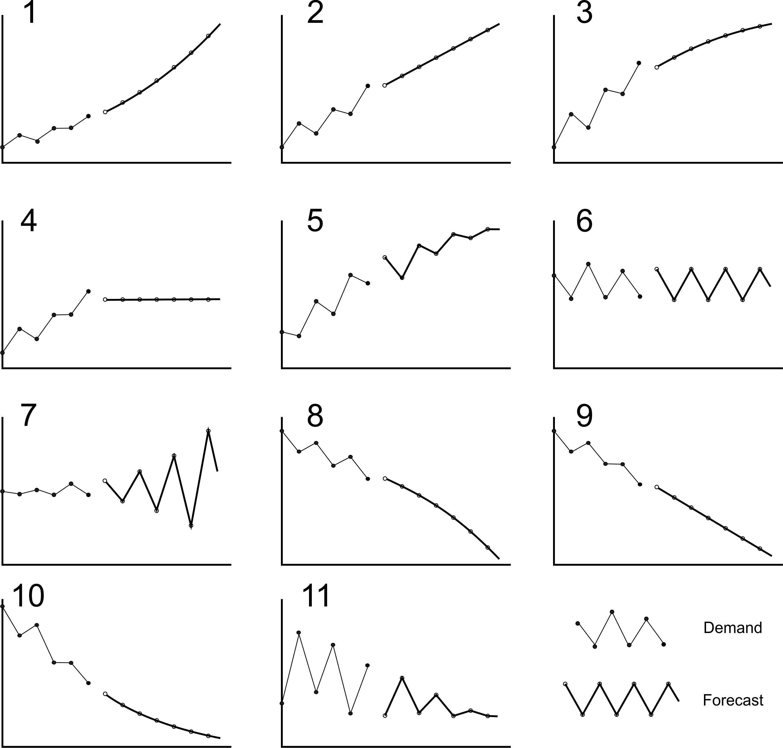
Figure 3.3: Illustrating the different Damped Trend responses
Table 3.7 provides an example calculation of the Damped Trend forecasts for the case when \(\alpha=0.5\), \(\beta=0.1\), and \(\phi=0.8\). Note, that the level, \(\hat{a}_t\), and trend, \(\hat{b}_t\), are different from those generated by the Holt’s method. Furthermore, the future forecasts \(\hat{d}_{t+n|t}\), the one period ahead forecasts when \(\phi=0.8\) are multiplied by \(\phi(\phi^1-1)/(\phi-1)=0.8\). The two period ahead forecast is multiplied by \(\phi(\phi^2-1)/(\phi-1)=1.44\). This multiple changes as \(n\), the number of periods ahead that we are forecasting, changes. When \(0 \leq \phi \leq 1\), the forecast changes with ever smaller increments in each period.
| Time, \(t\) | Demand, \(d_t\) | Forecast of the level, \(\hat{a}_t=(1-\alpha)\times\) \((\hat{a}_{t-1}+\phi\beta\hat{b}_{t-1})\) \(+\alpha d_2\) | Forecast of the trend, \(\hat{b}_t=\phi\hat{b}_{t-1}(1-\beta)\) \(+\beta(\hat{a}_t-\hat{a}_{t-1})\) | One period ahead forecast, \(\hat{d}_{t+1|t}=\hat{a}_t+\phi\hat{b}_t\) | Two periods ahead forecast, \(\hat{d}_{t+2|t}=\hat{a}_t+\) \((\phi+\phi^2)\hat{b}_t\) |
|---|---|---|---|---|---|
| \(1\) | \(10\) | \(\hat{a}_1=d_1=10\) | \(\hat{b}_1=0\) | \(\hat{d}_{2,1}=10\) | \(\hat{d}_{3,1}=10\) |
| \(2\) | \(6\) | \(\hat{a}_2=8\) | \(\hat{b}_2=-0.20\) | \(\hat{d}_{3,2}=7.84\) | \(\hat{d}_{4,2}=7.71\) |
| \(3\) | \(8\) | \(\hat{a}_3=7.92\) | \(\hat{b}_3=-0.15\) | \(\hat{d}_{4,3}=7.80\) | \(\hat{d}_{5,3}=7.70\) |
| \(4\) | \(12\) | \(\hat{a}_4=9.90\) | \(\hat{b}_4=0.09\) | \(\hat{d}_{5,4}=9.97\) | \(\hat{d}_{6,4}=10.03\) |
| \(5\) | \(10\) | \(\hat{a}_5=9.98\) | \(\hat{b}_5=0.07\) | \(\hat{d}_{6,5}=10.04\) | \(\hat{d}_{7,5}=10.09\) |
| \(6\) | \(14\) | \(\hat{a}_6=12.02\) | \(\hat{b}_6=0.29\) | \(\hat{d}_{7,6}=12.23\) | \(\hat{d}_{8,6}=12.39\) |
| \(7\) | \(12\) | \(\hat{a}_7=12.11\) | \(\hat{b}_7=0.19\) | \(\hat{d}_{8,7}=12.27\) | \(\hat{d}_{9,7}=12.39\) |
| \(8\) | \(8\) | \(\hat{a}_8=10.13\) | \(\hat{b}_8=-0.06\) | \(\hat{d}_{9,8}=10.09\) | \(\hat{d}_{10,8}=10.05\) |
| \(9\) | \(10\) | \(\hat{a}_9=10.04\) | \(\hat{b}_9=-0.05\) | \(\hat{d}_{10,9}=10.00\) | \(\hat{d}_{11,9}=9.97\) |
| \(10\) | \(10\) | \(\hat{a}_{10}=10.00\) | \(\hat{b}_{10}=-0.04\) | \(\hat{d}_{11,10}=9.97\) | \(\hat{d}_{12,10}=9.94\) |
Damped Trend contains other forecasting methods as specific cases, accessed by setting the parameters \(\alpha\), \(\beta\), and \(\phi\) to particular values. This effectively automates the forecast method selection problem. For example, Table 3.4 shows that Holt’s, Exponential Smoothing and Naïve methods are contained within the Damped Trend model. Thus, the Damped Trend is a good starting point for numerical investigations. The valid ranges of the Damped Trend parameters are complex; the following conditions must be satisfied:
The valid set of Damped Trend forecasting parameters. The following criteria must be met to produce stable damped trend forecasts.
- \(\phi-1<\alpha \phi<\phi+1\), and
- \(\alpha(\phi-1)<\alpha \beta \phi<(2-\alpha)(\phi+1)\).
It is probably best to incorporate these criteria into a spreadsheet to facilitate easy checking of the stability criteria (or use the interactive R-shiny webpage available here. Figure 3.4 provides a sketch of 12 different time series. After reading this Chapter to this point, you should now be able to determine a suitable forecasting technique for each time series. Have a go; the answers are given in Appendix C.
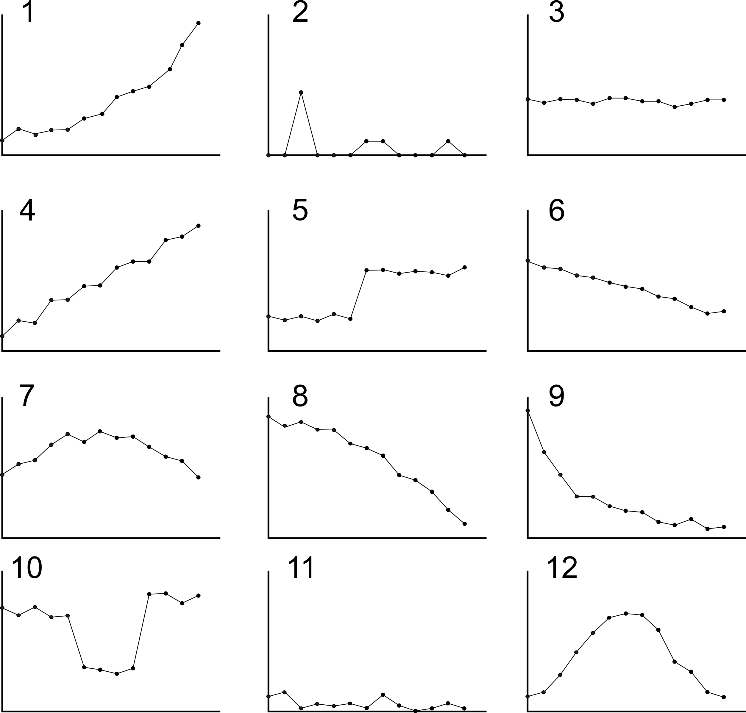
Figure 3.4: Forecasting method selection: Pop quiz
3.5 Tuning the forecasting parameters
Depending on your demand patterns, lead-times, replenishment policy choices, and cost structure of your business, you may have some idea about what forecasting strategy is suitable12.
| Forecasting method | Parameter setting | Notes |
|---|---|---|
| Holt’s Method | \(\phi=1\) | Setting \(\phi=1\) implies that \(\hat{d}_{t,t+k}=\hat{a}_t+k\hat{b}_t\). Future forecasts then become a linear extrapolation of the current estimate of the trend. |
| Exponential smoothing | \(\beta=0, \text{ }\phi=0\) | Setting \(\beta=0 \text{ and }\phi=1\) implies that \(\forall t\geq 0\), \(b_t=0\). It then follows that \(\hat{a}_t=(1-\alpha)\hat{a}_{t-1}+\alpha d_t\) and \(\hat{d}_{t,t+k}=\hat{a}_t\). |
| Naïve forecasting | \(\alpha=0, \text{ } \beta=0, \text{ }\phi=0\) | From the exponential smoothing formula, it is easy to see this parameter set results in \(\hat{d}_{t,t+k}=d_t\). |
The next task is to tune the forecasting parameters. We can do this by building up a model of the forecasting system in a spreadsheet, simulating the response of the forecasting system to some real demand data, and measuring its performance. By carefully evaluating performance (via some measures of forecasting performance that we will outline shortly) you will arrive at a set of forecasting parameters. Table 3.9 provides some good starting points in the parameter space for your investigations. Note, for naïve forecasts, there are no parameters to set. Parameter selection is probably best done in a manual, interactive, and iterative manner in a spreadsheet.13 Do not worry about forecast errors that are present in your simulation–there is no such thing a perfect forecast–forecasts are estimates of future demand of course they will have errors. The trick is to create a replenishment system that is robust in the sense that it mitigates the negative impact of the forecast errors. Chapter 4 covers replenishment system design.
| Forecasting method | Low volume demand | High-volume demands, short lead times | High-volume demands, long lead times |
|---|---|---|---|
| Moving average | \(n>25\) | \(2 < n< 10\) | \(5 < n< 25\) |
| Exponential smoothing | \(\alpha = 0.01\) | \(\alpha = 0.3\) | \(\alpha = 0.1\) |
| Holt’s method | \(\alpha = 0.1, \text{ } \beta=0.02\) | \(\alpha = 0.2, \text{ } \beta=0.05\) | \(\alpha = 0.1, \text{ } \beta=0.02\) |
| Damped trend | \(\alpha = 0.1, \text{ } \beta=0.02,\) \(\phi=0.9\) | \(\alpha = 0.2, \text{ } \beta=0.05\) \(\phi=0.9\) | \(\alpha = 0.1, \text{ }\beta=0.02\) \(\phi=0.9\) |
The following forecast performance measures can be used to evaluate your forecasting system. It is probably best to simulate this offline in Excel. Your simulation is a safe, risk-free environment to search for suitable values of the forecast parameters based on your demand patterns, cost structures, lead-times, etc. When you have identified some potentially useful parameter values, you can use them online in your ERP system to automatically generate forecasts each week. Note that, while we use the forecasting measures of performance to identify forecasting parameters, you still need to qualitatively evaluate the forecasting system to determine if it operates is as expected and it fits with your value stream setting.
Measures of forecast performance
- Bias. A measure of the forecasts ability to track long-term trends in demand. Bias can be positive and negative, and the closer it is to zero, the better.
- Variance of the \(n\)-period ahead forecast error. If we could predict precisiely the demand in the period after the lead time, we would not need any inventory, as supply would prefectly match demand. This measure should be minimised when only inventory only costs are present.
- Variance of the sum of the forecast errors over the lead-time and review period. In the OUT replenishment policy (and the Pure Pull policy) this is exactly equal to the variance of the inventory levels. In setting where we wish to minimise inventory costs only, then this measure should be as small as possible.
- Variance of the \(n\)-period ahead forecast. The n-period ahead forecast is added directly into the production/replenishment order by the OUT policy. Thus, the variance of the n-period-ahead forecast strongly influences Bullwhip and the capacity costs generated by the system. This metric should be minimised if we wish to reduce Bullwhip and capacity costs.
- Variance of the change in the \(n\)-period ahead forecasts. Some demands and forecasts change slowly (easy to forecast and to produce to) and others are more erratic and change quickly (harder to forecast and to produce to); they may even have the same variance. This measure measures the rate of change in the forecasts and should be minimised to reduce Bullwhip and capacity costs.
Bias. Bias is a term related to the ability of a forecast (\(n\) periods ahead) to predict the long term average of the time series (presumably demand). Mathematically it is defined as,
\[\begin{align} \tag{3.1} b_n=\mathbb{E}[\hat{d}_{t+n|t}]-\mathbb{E}[d_{t+n}]=\frac{1}{j-n} \sum_{t=1}^{j-n}(\hat{d}_{t+n|t}-d_{t+n}), \end{align}\]
showing that the bias, \(b_n\), is the expected (or average) forecast minus the expected (average) demand. The variable \(j\) is the number of demand points in your time series.
For a viable forecasting methodology, the forecast should be unbiased. That is, \(b_n\) should be zero. In practical situations, \(b_n\) may not be zero (even with an unbiased system), but as the number of data points \((j-n)\) used to calculate \(b_n\) increases, \(b_n\) should approach zero. If \(b_n>0\) \((b_n<0)\) for extended periods then the forecasts may be consistently over- (or under-) estimating the demand. Table 16 highlights how to calculate the one, two, and three periods-ahead forecast bias. For example, the one period ahead forecasting bias is \(b_1=0\), the two periods ahead forecast bias is \(b_2=-0.5\) and the three-period bias, \(b_3=-0.85.\)
| Time, \(t\) | Demand, \(d_t\) | Forecast of demand, \(\hat{d}_{t+n|t}\) | One period ahead error, \(\hat{d}_{t+1|t}-d_{t+1}\) | Two periods ahead error, \(\hat{d}_{t+2|t}-d_{t+2}\) | Three periods ahead error, \(\hat{d}_{t+3|t}-d_{t+3}\) |
|---|---|---|---|---|---|
| 1 | 10 | 10 | \(\hat{d}_{2,1}-d_2=4\) | \(\hat{d}_{3,1}-d_3=2\) | \(\hat{d}_{4,1}-d_4=-2\) |
| 2 | 6 | 8 | \(\hat{d}_{3,2}-d_3=0\) | \(\hat{d}_{4,2}-d_4=-4\) | \(\hat{d}_{5,2}-d_5=-2\) |
| 3 | 8 | 8 | \(\hat{d}_{4,3}-d_4=-4\) | \(\hat{d}_{5,3}-d_5=-2\) | \(\hat{d}_{6,3}-d_6=-6\) |
| 4 | 12 | 10 | \(\hat{d}_{5,4}-d_5=0\) | \(\hat{d}_{6,4}-d_6=-4\) | \(\hat{d}_{7,4}-d_7=-2\) |
| 5 | 10 | 10 | \(\hat{d}_{6,5}-d_6=-4\) | \(\hat{d}_{7,5}-d_7=-2\) | \(\hat{d}_{8,5}-d_8=2\) |
| 6 | 14 | 12 | \(\hat{d}_{7,6}-d_7=0\) | \(\hat{d}_{8,6}-d_8=4\) | \(\hat{d}_{9,6}-d_9=2\) |
| 7 | 12 | 12 | \(\hat{d}_{8,7}-d_8=4\) | \(\hat{d}_{9,7}-d_9=2\) | \(\hat{d}_{10,7}-d_10=2\) |
| 8 | 8 | 10 | \(\hat{d}_{9,8}-d_9=0\) | \(\hat{d}_{10,8}-d_{10}=0\) | - |
| 9 | 10 | 10 | \(\hat{d}_{10,9}-d_{10}=0\) | - | - |
| 10 | 10 | 0 | - | - | - |
| Average | \(b_1=0\) | \(b_2=-0.5\) | \(b_3=-0.85714\) |
The variance of the \(n\)-period ahead forecast error. The variance of the \(n\)-period-ahead forecast error is a measure of forecast accuracy. It is defined as,
\[\begin{align} \tag{3.2} \sigma^2_{fe,n}=\frac{1}{j-n}\sum_{t=1}^{j-n}(\hat{d}_{t-n|t}-d_{t-n})^2, \end{align}\]
where the variance of forecast error is given by the average squared forecast error \((\hat{d}_{t+n|t}-d_{t+n})^2\). Actually, here we are calculating the mean squared forecast error n-periods ahead. However, I have elected to call to the variance of the forecast error n-periods ahead as when the forecasts are unbiased, the mean squared forecast error is equal to the variance of the forecast error. Plus, the variance moniker is more easily associated with the Bullwhip and NSAmp ratios. Table 3.11 provides a detailed calculation of the variance of the forecast error.
| Time, \(t\) | Demand, \(d_t\) | Forecast of demand, \(\hat{d}_{t+n|t}\) | One period squared forecast deviation, \((\hat{d}_{t+1|t}-d_{t+1}-b_1)^2\) | Two period squared forecast deviation, \((\hat{d}_{t+2|t}-d_{t+2}-b_2)^2\) |
|---|---|---|---|---|
| \(1\) | \(10\) | \(10\) | \((10-6)^2=16\) | \((10-8)^2=4\) |
| \(2\) | \(6\) | \(8\) | \((8-8)^2=0\) | \((8-12)^2=16\) |
| \(3\) | \(8\) | \(8\) | \((8-12)^2=16\) | \((8-10)^2=4\) |
| \(4\) | \(12\) | \(10\) | \((10-10)^2=0\) | \((10-14)^2=16\) |
| \(5\) | \(10\) | \(10\) | \((10-14)^2=16\) | \((10-12)^2=4\) |
| \(6\) | \(14\) | \(12\) | \((12-12)^2=0\) | \((12-8)^2=16\) |
| \(7\) | \(12\) | \(12\) | \((12-8)^2=16\) | \((12-10)^2=4\) |
| \(8\) | \(8\) | \(10\) | \((10-10)^2=0\) | \((10-10)^2=0\) |
| \(9\) | \(10\) | \(10\) | \((10-10)^2=0\) | \(-\) |
| \(10\) | \(10\) | \(10\) | \(-\) | \(-\) |
| Average | \(\sigma^2_{fe,1}=7.11\) | \(\sigma^2_{fe,2}=8\) |
The variance of the sum of the forecast errors over the lead-time and review period. When using the order-up-to policy the safety stock requirements are linearly related to the standard deviation of the sum of the forecast errors over the lead-time and review period. Thus minimizing the variance of the sum of the forecast errors over the lead-time and review period, leads to minimum inventory variance and minimum inventory costs.
\[\begin{align} \tag{3.3} \sigma^2_{\Sigma\hat{d}}=\frac{1}{j-T_p-1}\sum_{t=1}^{j-T_p-1}\left(\mu_{\Sigma \hat{d}}-\sum_{n=1}^{T_p+1}\left(\hat{d}_{t+n|t}-d_{t+n}\right)\right)^2 \end{align}\] where \[\begin{align} \tag{3.4} \mu_{\Sigma \hat{d}}=\left(\sum_{t=1}^{j-T_p-1}(\hat{d}_{t+n|t}-d_{t+n}\right)\bigg/ (j-T_p-1). \end{align}\]
The forecasts in periods \(n=\{1,2,...,T_p\}\) are required to be accurate to set the desired work-in-progress level correctly. The forecast accuracy \(T_p+1\) periods ahead directly influences the inventory (safety stock) requirements. If the forecast \(T_p+1\) periods ahead were entirely accurate then (in the OUT policy), there would be no need for inventory and variance of the orders would equal the variance of the demand.
To calculate the variance of the forecast errors over the lead-time and review period Table 3.12 shows that we first determine the sum of the forecast errors over the lead time review period in each period. Here we have assumed that the lead-time \(T_p=1\). Thus, we subtract the sum of forecasts for the next period and the next, next period from the sum of the demand in the next period and the next, next period. The then find the average of those forecast errors, \(\mu_{\Sigma \hat{d}}\). We then average the squared difference between the errors and the mean error to obtain the variance (mean squared error) of the forecast error over the lead-time and review period, \(\sigma^2_{\Sigma\hat{d}}\).
| Time, \(t\) | Demand, \(d_t\) | Forecast of demand, \(\hat{d}_{t+n|t}\) | Sum of the forecast errors over lead-time and review period \(d_{t+1}+d_{t+2}-2\hat{d}_{t+n|t}\) | Squared forecast error, \[(\mu_{\Sigma \hat{d}}-(d_{t+1}+\\ d_{t+2}-2\hat{d}_{t+n|t}))^2\] |
|---|---|---|---|---|
| \(1\) | \(10\) | \(10\) | \(6+8-(2\times 10)=-6\) | \((-6.5)^2=42.25\) |
| \(2\) | \(6\) | \(8\) | \(8+12-(2\times 8)=4\) | \(3.5^2=12.25\) |
| \(3\) | \(8\) | \(8\) | \(12+10-(2\times 8)=6\) | \(5.5^2=30.25\) |
| \(4\) | \(12\) | \(10\) | \(10+14-(2\times 10)=4\) | \(3.5^2=12.25\) |
| \(5\) | \(10\) | \(10\) | \(14+12-(2\times 10)=6\) | \(5.5^2=30.25\) |
| \(6\) | \(14\) | \(12\) | \(12+8-(2\times 12)=-4\) | \((-4.5)^2=20.25\) |
| \(7\) | \(12\) | \(12\) | \(8+10-(2\times 12)=-6\) | \((-6.5)^2=42.25\) |
| \(8\) | \(8\) | \(10\) | \(10+10-(2\times 10)=0\) | \(0.5^2=0.25\) |
| \(9\) | \(10\) | \(10\) | \(-\) | \(-\) |
| \(10\) | \(10\) | \(10\) | \(-\) | \(-\) |
| Average | \(\mu_{\Sigma \hat{d}}=0.5\) | \(\sigma^2_{\Sigma\hat{d}}=23.75\) |
The variance of the forecast. Minimizing the forecast error assumes that only inventory-related costs (holding and backlog/shortage) exist and production is infinitely flexible at no cost. However, in the OUT/POUT policy, the \(T_p+1\) periods ahead forecast is added directly into the order rate with no smoothing or filtering. Thus, variability in the demand forecast adds to the order variability. Variable orders could be expensive in situations with high Muri and Mura costs. So we should also measure the variance of the forecast, \[\begin{align} \sigma^2_{\hat{d}}=\mathbb{V}[\hat{d}_{t+n|t}]=\frac{1}{j} \sum_{t=1}^j (\mu_{\hat{d}}-\hat{d}_{t+n|t})^2, \end{align}\] where \(\mu_{\hat{d}}= \frac{1}{j} \sum^j_{t=1} \hat{d}_{t+n|t}.\)
The forecast variability measure is often in conflict to the accuracy measure, and unless the demand is constant, then a forecast cannot have zero error variance and zero forecast variance simultaneously. Furthermore, because the variance of the \(T_p+1\) period ahead forecast is added directly into the replenishment/production orders, there is a trade-off between inventory forecast requirements and the Bullwhip forecasts requirements. Minimizing \(\sigma^2_{\hat{d}}\) reduces Bullwhip, but minimizing \(\sigma^2_{fe}\) reduces inventory costs.
An example of the procedure to calculate the variance of the \(n\)-period-ahead exponential smoothing forecasts are given in Table 3.13. Note that all future forecasts produced by the exponential smoothing forecasting mechanism are identical, so we don’t have to account for the number of periods ahead, \(n\), that we are forecasting. If the forecasts do change over the forecast horizon, as they do for Holt’s and damped trend, we would need a measure of forecast variability for each \(n\).
| Time, \(t\) | Demand, \(d_t\) | Forecast of demand, \(\hat{d}_{t+n|t}\) | Squared forecast deviation, \((\mu_{\hat{d}}-\hat{d}_{t+n|t})^2\) |
|---|---|---|---|
| 1 | 10 | 10 | \((10-10)^2=0\) |
| 2 | 6 | 8 | \((10-8)^2=4\) |
| 3 | 8 | 8 | \((10-8)^2=4\) |
| 4 | 12 | 10 | \((10-10)^2=0\) |
| 5 | 10 | 10 | \((10-10)^2=0\) |
| 6 | 14 | 12 | \((10-12)^2=4\) |
| 7 | 12 | 12 | \((10-12)^2=4\) |
| 8 | 8 | 10 | \((10-10)^2=0\) |
| 9 | 10 | 10 | \((10-10)^2=0\) |
| 10 | 10 | 10 | \((10-10)^2=0\) |
| Average | \(\mu_{\hat{d}}=10\) | \(\sigma^2_{\hat{d}}=1.6\) |
Variance of the change in the \(n\)-period ahead forecasts. Changing the production rate from period to period is costly, so we may wish to minimize the variance of the change in the forecast from period to period. A relevant measure is
\[\begin{equation} \sigma^2_{\Delta\hat{d}}=\mathbb{V}[\hat{d}_{t+n|t}-\hat{d}_{t+n-1|t-1}]=\frac{1}{j-n}\sum_{t=1}^{j-n}(\mu_{\Delta\hat{d}}-\hat{d}_{t+n|t}-\hat{d}_{t+n-1|t-1})^2 \end{equation}\]
where \(\mu_{\Delta \hat{d}}=\frac{1}{j-n} \sum_{t=1}^{j-n} (\hat{d}_{t+n|t}-\hat{d}_{t+n-1|t-1})\). \(\sigma^2_{\Delta \hat{d}}\) gives an indication of how quickly the forecasts are changing. When all other measures are equal, slowly changing forecasts are more desirable than rapidly changing forecasts. See Figure 3.5 where each of the three lines has the same variance (as they contain the same numbers, just ordered in time differently), but very different variances of the change in the forecast. Smaller forecast change variance facilitates more efficient production. Table 3.15 details the calculations required to determine the variance of the forecast change. We note that in the last \(T_p+1\) periods, as there is no known demand, the difference between the current forecast and the previous forecasts cannot be calculated.
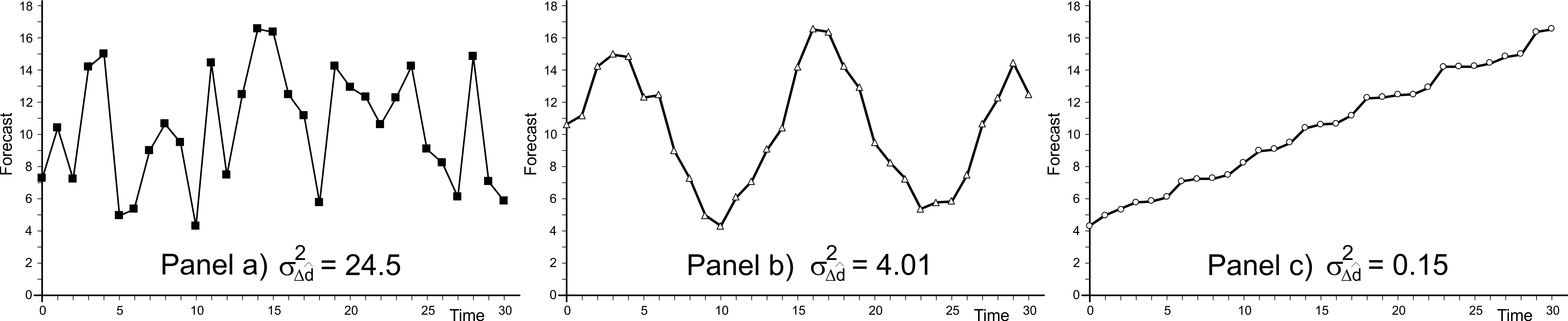
Figure 3.5: Three forecasts with identical forecast variance but different variances of forecast change
| Time, \(t\) | Demand, \(d_t\) | Forecast of demand, \(\hat{d}_{t,t+n}\) | Change in the forecast, \(\hat{d}_{t+n|t}-\hat{d}_{t+n-1|t-1}\) | Squared forecast change deviation, \((\mu_{\Delta\hat{d}}-\hat{d}_{t+n|t}-\hat{d}_{t+n-1|t-1})^2\) |
|---|---|---|---|---|
| \(1\) | \(10\) | \(10\) | \(-\) | \(-\) |
| \(2\) | \(6\) | \(8\) | \(8-10=-2\) | \((0-(-2))^2=4\) |
| \(3\) | \(8\) | \(8\) | \(8-8=0\) | \((0-0)^2=0\) |
| \(4\) | \(12\) | \(10\) | \(10-8=2\) | \((0-2)^2=4\) |
| \(5\) | \(10\) | \(10\) | \(10-10=0\) | \((0-0)^2=0\) |
| \(6\) | \(14\) | \(12\) | \(12-10=2\) | \((0-2)^2=4\) |
| \(7\) | \(12\) | \(12\) | \(12-12=0\) | \((0-0)^2=0\) |
| \(8\) | \(8\) | \(10\) | \(10-12=-2\) | \((0-(-2))^2=4\) |
| \(9\) | \(10\) | \(10\) | \(10-10=0\) | \((0-0)^2=0\) |
| \(10\) | \(10\) | \(10\) | \(10-10=0\) | \((0-0)^2=0\) |
| Average | \(\mu_{\Delta\hat{d}}=0\) | \(\sigma^2_{\Delta\hat{d}}=1.77\) |
In summary, measures of forecast performance should be carefully selected to match the supply chain requirements, see Table 3.15.
| Supply chain measure | Bias | Variance of forecast error | Variance of the sum of forecast errors over lead time and review period | Variance of the forecast | Variance of the change in forecast |
|---|---|---|---|---|---|
| Inventory costs | Close to zero | Minimise as second priority | Minimise as first priority | No influence | No influence |
| Customer service level | Close to zero | Minimise as second priority | Minimise as first priority | No influence | No influence |
| Bullwhip costs | Close to zero | No influence | No influence | Minimise as first priority | Minimise as second priority |
 A Shiny App is available here where you can explore the dynamic consequences of naïve, exponential smoothing, Holts method and damped trend forecasting interactively. You can upload you own demand time series, measure the forecast performance, select forecasting methods, and identify suitable forecasting parameters.
3.6 Manual interventions
Many companies have a forecasting team that is responsible for making manual adjustments to computer-generated forecasts to improve forecast accuracy, see Figure 3.6. No computerized systems will have the knowledge and experience of all the real world issues that we, as humans, can recognize and manage. Thus, manual interventions into the forecasting system will occasionally be required. However, human judgement is often subject to bias and inconsistency.
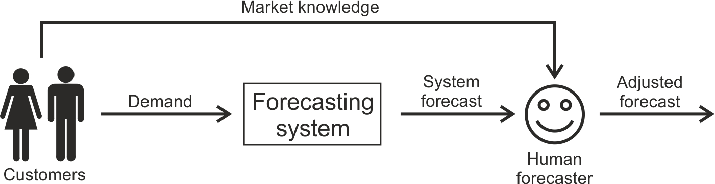
Figure 3.6: Schematic of a human judgemental forecast adjustment
Typical human forecasting biases include:
Common human forecasting biases
- Company politics. The forecast reflects what the boss wants to hear or some other agenda. For example, your manager may wish to see 10% sales growth and the forecasts to reflect that, or perhaps you want to employ more staff and so future forecasts are inflated to increase the chance of approval.
- Overconfidence. Perhaps you are over-confident in the new sales team or the demand for a new product.
- Wishful thinking. People are prone to make overly optimistic forecasts.
- Success/failure attribution. People are likely to assign the cause of accurate forecasts internally to themselves (they are intelligent, skillful, insightful, knowledgeable of the situation). However, poor forecasts are assigned to external causes (bad luck, poor weather, competitor activity).
- The gambler`s fallacy. Good and bad luck will cancel each other out in the long run, or the universe has a memory.
- Conservatism. People often refuse to accept radical change.
- Data presentation. Misleading graphs and tables are too readily accepted.
The problem with manually adjusting forecasts is that people tend to meddle excessively. For example, forecasters like to make changes to every product, in every period despite having no good reason to do so. Perhaps they need to feel like they are in control, or perhaps they need to convince themselves (or their manager) they are attending to the task. However, small increases or decreases to systematic forecasts do not make a significant improvement to the forecast accuracy (because the changes are small) and, more often than not, actually make it worse. In contrast, substantial manual reductions to forecasts usually result in a significant improvement in the forecast accuracy. The reason for this may be that the human forecast adjustments have been made in light of market knowledge (maybe a new product has been introduced, a new competitor has arrived in the market, or the selling season ends). However, large increases to forecasts usually reduce forecast accuracy. Perhaps because increases in demand are naturally harder to predict, or perhaps because forecast increases have been made for some other reason such as meeting a budget, motivating a sales force, or stock building, for example.
Automatic, algorithmic forecasts are almost always more accurate than humans and are cheap and easy to create. Past demand history can be used to create the forecasts. That said, there is a time when human intervention is required. For example, perhaps it is known that demand for a product will significantly decrease when a new updated version is introduced. Maybe, at the end of a product’s life cycle, the number of production sites making the product will be reduced, and the factories where demand is transferred too will see an increase in demand (in this case we may want to manipulate the past demand data used to make the remaining forecasts). Perhaps we know that the customer will be on holiday for the next few weeks and there will be no demand. The point is that human judgement is required to maintain a good set of forecasts, but if the forecasting system is set up correctly, the intervention required will be concerned with dealing with the exceptions, the special situations, the one-off issues. The day-to-day operation of the forecasting system should be mostly automatic and free from human intervention.
When to manually adjust your forecasts
- During periods of holidays, plant shutdowns and maintenance.
- Changing the source of supply.
- Consolidating part number and product ranges.
- Introduction of the next generation of products.
- Significant competitive/market changes.
- Promotion, seasonal, and weather-related demand changes.
- End of life issues, all time builds.
3.7 Implementation issues
It may be helpful to categorize your products into a smaller number of forecasting groups. For example, the following categories will allow you to manage the forecasting parameters for a large number of products:
- Low volume or intermittent production.
- High volume, short lead-time.
- High volume, long lead-time.
However, as the demand profile changes over the product’s life-cycle, you will need to periodically review which category is most suitable for each product in your portfolio.
The initial conditions can have a long-term impact on the forecasts (the further you are away from the initial conditions, the better, but they can still have an impact). If the starting point changes each week, then the initial conditions can produce forecasts that fluctuate from week to week, especially when there is only a small amount of historical data present (especially when Holt’s or damped trend is used). It is better to fix the start week and adjust the data in this period so that a reasonable set of initial conditions are used, helping to create more stable forecasts. Running the forecasting module in your ERP for a few weeks before using its output in the next stage of the production planning cycle–the planning book–will allow the forecasting algorithm to find its internal levels and trends. You can also use this time to validate your forecasting methodology and gain confidence in your progress.
Remember, no forecasting method will ever be able to perfectly predict demand in the future. Every demand pattern will have its own level of achievable forecast accuracy - this is the most accurate forecasts that are possible. As forecast accuracy costs time and effort too improve and having more accurate forecasts have only a limited economic benefit, there is also the concept of desirable level of forecast accuracy. If the achievable forecasts accuracy is less than the desirable forecast accuracy, you have three options:
- Increase safety stocks (as safety stock can absorb the forecast errors).
- Decrease the lead time by shortening the production cycle, using faster transportation modes, or selecting closer suppliers.
- Manage the customer’s demand in some way so that it becomes more forecastable.
Finally, let us summarize our forecasting discussion by considering Figure 3.7. Here we have forecasts, made now at the very end of period \(t\), of demand in period \(t + n\) where the lead-time \(T_p=3\). Thus the forecast of the demand over the lead-time is the sum of the forecasts for \(n = 1, 2,\) and \(3\). The next forecast (when \(n = 4\)) is the forecast of demand in the period after the lead-time. These two forecasts are used in the next Chapter 4 to set production and distribution targets. The forecasts of demand in the future (\(n = 5, 6, 7, 8, ...\)) are used in the MRP module to provide ourselves, and our suppliers, with some guidance of likely future demand. This future guidance is used in long-term capacity planning activities and is the focus of Chapter 6.
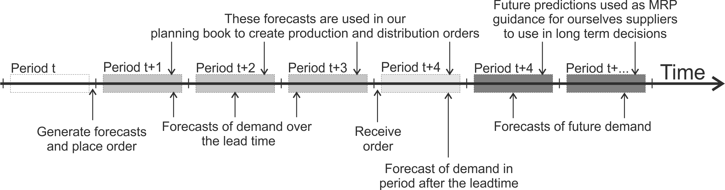
Figure 3.7: Use of forecasts when lead-time \(T_p=3\)
Or other relevant software if you use a specialized forecasting application.↩︎
We could have also included a seasonal forecasting methodology (such as Holt’s-Winters) in this list as well as a forecasting method for intermittent demand (such as Croston’s Method). For the sake of brevity these have been omitted.↩︎
Many forecasting experts advocate that \(0 \leq \alpha \leq 1\), but I prefer to recommend the full range of stable \(\alpha\)’s even though \(\alpha>1\) are practically rare.↩︎
To back-cast, reverse the order of the time series and forecast that new series to find the initial forecast in the original time series.↩︎
Actually, strictly speaking it decreases geometrically, not exponentially, but this is the accepted terminology.↩︎
It may be the case that some product/customer location pairs use one particular forecasting method and another product/customer location pair uses a different another method.↩︎
I have created an interactive R-shiny website hosted here for you to use as a starting point in your own investigations. It has the naive, exponential smoothing, Holt’s and damped trend forecasting methods and the supply chain measures of performance pre-coded. All you will need to do is load your own demand data and you can use the shiny to identify good forecasting parameters.↩︎