Chapter 4 Planning book: Setting the cadence of your pacemaker

Figure 4.1: This chapter is currently under construction, it will probably be ready in week 4 or 5 of the semester. Please come back later

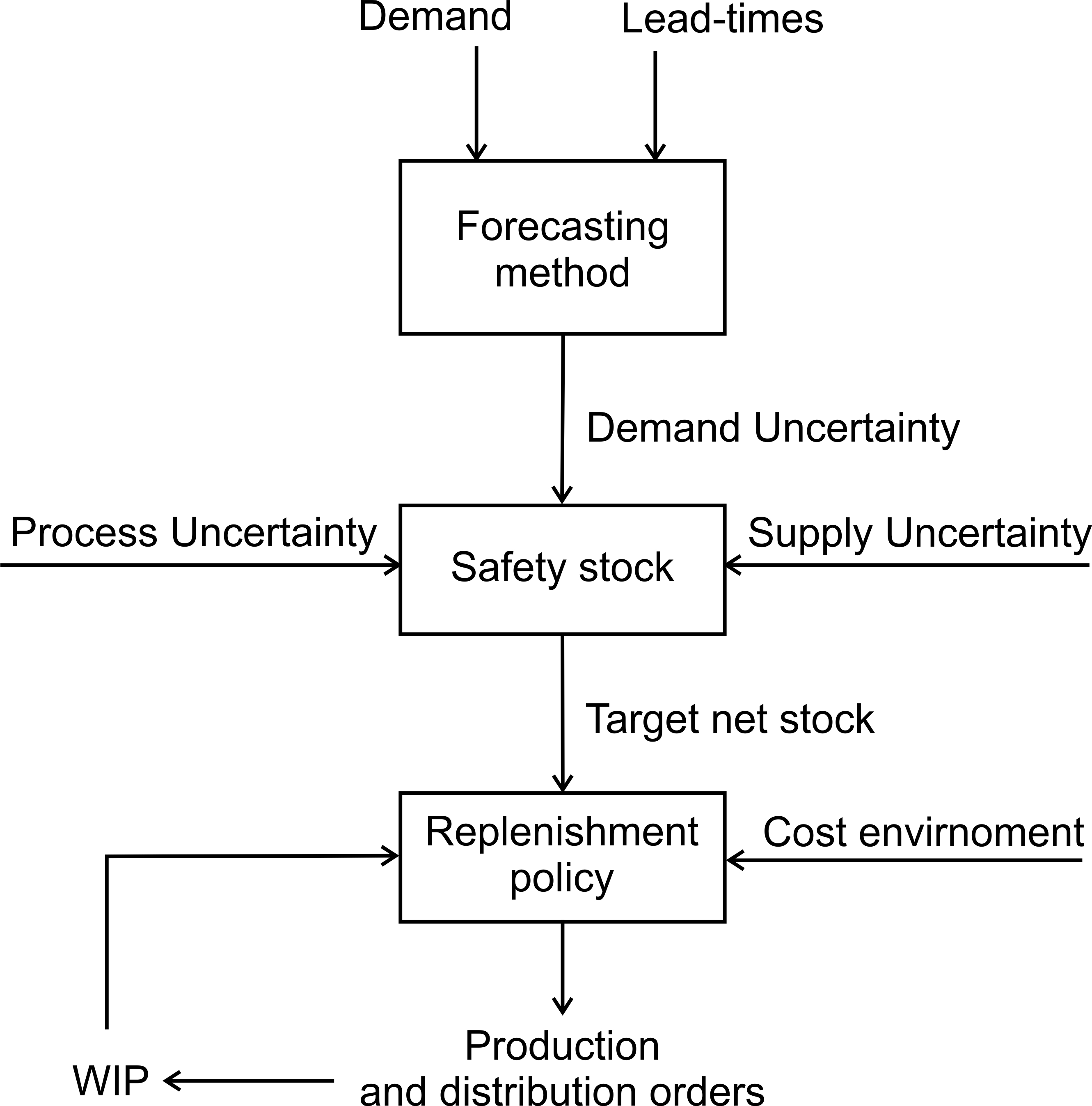
The forecasting module has made predictions about the demand in future periods. The next task is to net the forecasts and demand against the inventory and work-in-progress, account for the lead-time, and set production and distribution targets. Depending on your preferred replenishment strategy for your value stream, you now need to design your replenishment policy. This may seem like a rather daunting task (it is), but fortunately, the POUT replenishment policy is available and can be tuned to mimic all of the replenishment policies, see Table 4.1. In a sense, it is like the Swiss army knife of replenishment policies as the POUT policy offers a very efficient solution procedure. First, adapt your existing OUT based replenishment system to become a POUT system. Then, tune the POUT policy to realize your desired replenishment strategy.

Table 4.1: Tuning the POUT policy to match your replenishment strategy

Strategy	How to tune the POUT policy
Pure Pull: Produce to the current demand rate (from either your immediate customer or from the end consumer)	Set \(T_i=1\) and use a constant forecast
Level Scheduling: Produce to average demand (with/without periodic changes in the safety stocks or number of kanbans)	Set \(T_i=\infty\) and use a constant forecast set to the true mean of the demand
Forecast: Produce to a forecast	Set \(T_i=\infty\) and use a dynamic forecast
Batch: Produce an Economic Production Quantity	Set \(T_i=1\) and use a dynamic forecast plus an Economic Production Quantity
Order-up-To: Produce to a forecast and fully account for inventory and WIP discrepancies.	Set \(T_i=1\) and use a dynamic forecast
Proportional Order-Up-To: Produce to a forecast and only account partially for inventory and WIP discrepancies	Set \(T_i\geq1\) and use a dynamic forecast

4.1 The sequence of events

Assume Acme Ltd plans its production and distribution on a weekly basis as shown in Figure 4.2. At 23.59 Sunday night, the week’s demand is tallied by the ERP system, inventory and WIP (in-transit inventory) levels are observed, a demand forecasts are generated, and a production and distribution plan is created. The Monday morning production planning meeting then confirms the production and distribution targets for the week. Detailed scheduling also takes place that accounts for changeover costs between products, shipping schedules, and maintenance activities. A time-phased production plan is then sent to the factory floor.

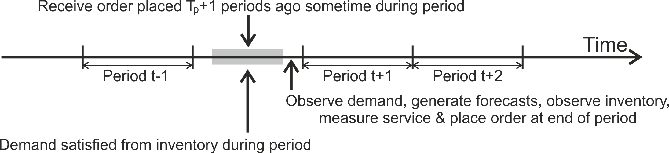
Figure 4.2: The sequence of events in a production planning system

Note, even if the physical lead time is instantaneous, the products ordered will only be received and be ready to satisfy demand in the next period; the consequences of this would not be considered until the next order is placed (at the end of the following period). Further note, if the replenishment orders were placed at the very beginning of a period, it would still be based on the same information as an order was placed at the very end of the previous period; all that changes is the time index of the state variables (the inventory, orders, WIP, and forecasts are the state variables).

4.2 The lead time

Before we review the different production planning approaches, first we consider the meaning of a lead time as it is a major component of a production planning algorithm. Simply put, the lead time is the period of time between generating a production order to the time that order is received in FGI (or VMI). If you have a constant, known, consistently and correctly recorded lead time then you are very lucky as this simplifies the planning problem.

The lead time includes the time to place an order, manufacture product, pack, assemble shipment, ship, transport, and receive that product into a stock location. There will be many instances where a lead time is defined in an ERP system. For example, lead time information will be defined, stored, and used in the planning book, supplier contracts and purchasing ledgers, transport routes, and the master bill of materials (BOM) file. Different functions (departments, people) will have responsibility and access/permission to keep that information up-to-date. For example, the production planning team may control the planning book, the purchasing team may set up supplier relationships in the contract files and purchasing ledgers, the transport managers select shipping companies and routes, engineering/design define the BOM. All this lead time information has to be coordinated. Amazingly, most ERP do not have a single global variable for a lead time; there are many instances of this variable and they could be different. Synchronizing lead time information may mean that several fields within your ERP system will need to be checked and possibly corrected. Furthermore, as many people will likely have the opportunity and authority to change lead-time information, ERP lead times changes need to be coordinated in some way. Communicating with, and gaining the necessary buy-in from, all the stakeholders with an interest in lead time changes might be a difficult task, but it is essential for proper supply chain control, see Figure 4.3. The challenge is to find a lead time updating protocol that is not unduly slow and burdensome.

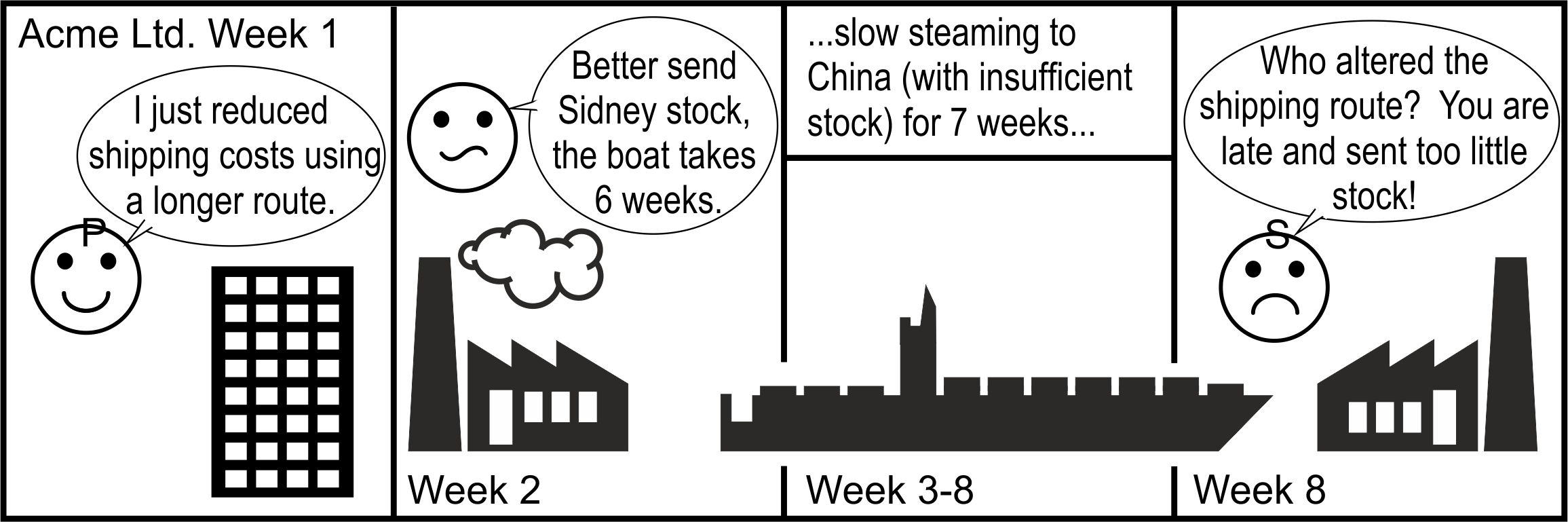
Figure 4.3: Decisions taken by one part of the value stream need to be communicated to many other parts

There are many factors that affect the actual physical lead times: 1) natural variability of the lead times resulting from factors such as the weather, congestion, and customs delays, 2) seasonal variability, 3) special causes. Figure 4.4 provides an example of real lead times in two forms; the lead time that was quoted by the freight forwarding company at the time of dispatch and the actual lead time recorded when the shipment was received. We can see from Figure 4.4 the quoted lead time is a variable itself. It experiences seasonal effects (December and January have higher quoted lead-times). The actual lead times are more consistent, but still variable. Interestingly, throughout 2008, most of the actual lead times were longer than the quoted lead time. However, for the period from June 2009 through 2010, most actual lead times were shorter than the quoted lead time. This may be due to factors outside of the shipping company’s control; bad weather, berth availability at ports, custom delays, lack of transportation capacity for hinterland distribution, for example. However, it should be clear that you should monitor the actual lead times yourself and keep a good record of what is actually happening.

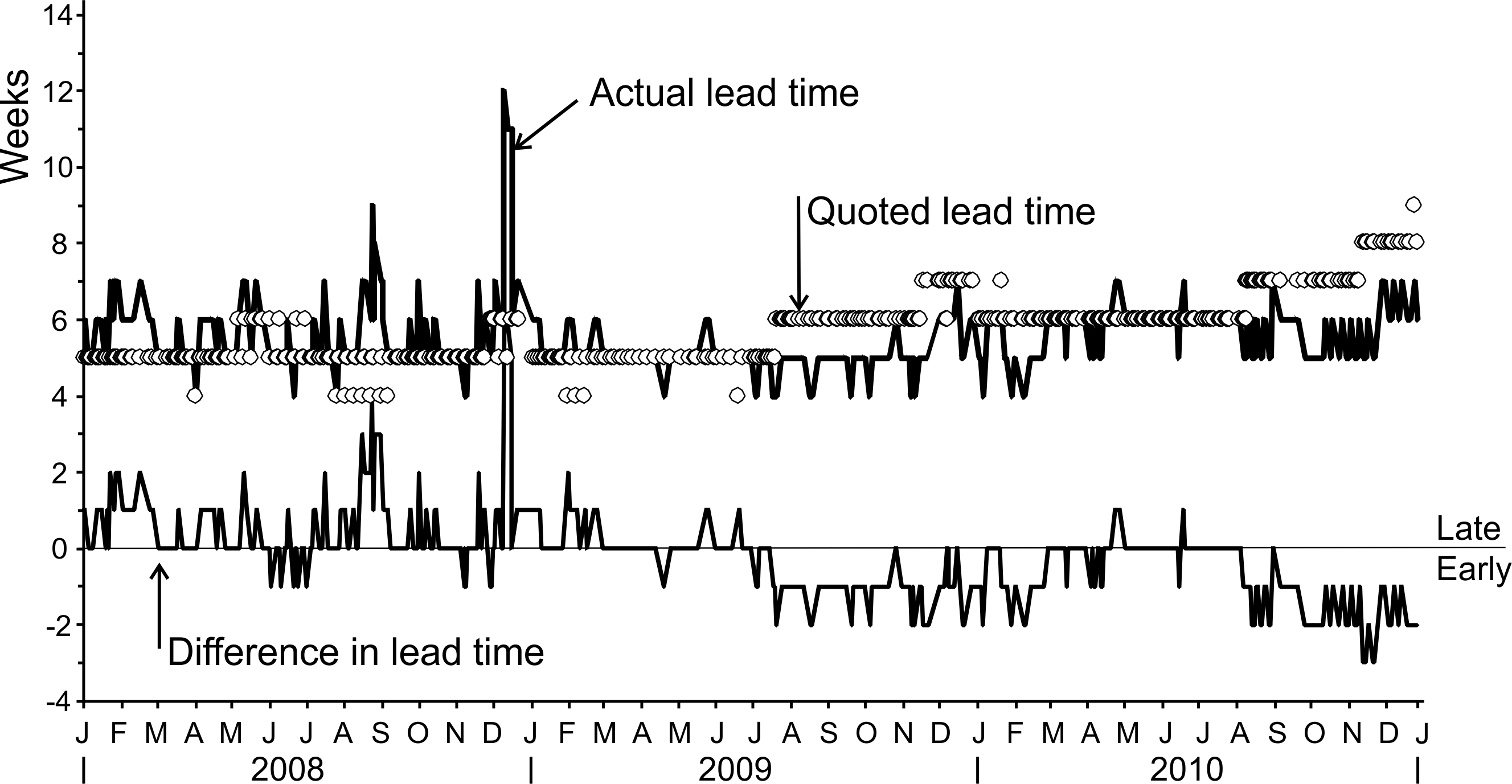
Figure 4.4: The quoted and actual lead-times in a global shipping lane

The consequences of incorrectly specified lead times can be quite severe. If the perceived lead time is longer (shorter) than the actual lead time then excessive (insufficient) inventory will be held. If the lead time used in the planning book and the OUT policy is used to schedule production, then the supply chain will become both unstable and chaotic as the OUT policy requires accurate lead time information, Wang, Disney, and Wang (2012). A properly tuned POUT policy will, however, remain stable and will not produce chaotic responses if incorrect lead times exist; a significant advantage of the POUT policy, Disney et al. (2016). If a stochastic lead time is present then it is important that the average lead time is used in your replenishment decision, see Figure 4.5. This ensures that inventory does indeed fluctuate around the target safety stocks levels and customer service levels are achieved. It is important that a long-term average lead time is used as dynamically forecasting lead times can produce massive amounts of bullwhip. This can be determined from the probability mass function (PMF) of previous lead-times (see Michna, Disney, and Nielsen (2019) for insights into the consequences of forecasting stochastic lead times). In the next section we consider how to correctly identify a lead time from real life lead time data and the PMF of previous orders.

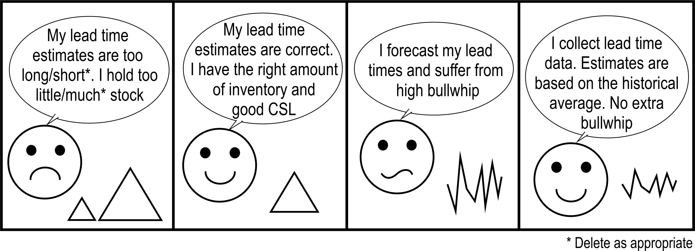
Figure 4.5: It is important to indetify and use the correct average lead time

4.2.1 Determining the lead time in a periodic replenishment system

Lead time estimates have a large impact on the dynamic behaviour and stability of a replenishment system. It is important that the average lead time parameters in ERP/replenish algorithms match the average real life lead-time. We need a procedure to monitor, track, and update the lead time information every 3-6 months. This will probably involve creating a spreadsheet where actual replenishment orders (to suppliers) and production targets (to our production system) are recorded. The length of lead-time for each production order needs to be recorded, before determining the average lead-time. The average lead time is likely to be a real valued number, but the discrete time nature of the OUT and POUT policy requires integer valued lead times. The following call-out and exercise describes how to convert physical lead times into the integer lead-times required by an ERP system.

Lead time settings in ERP systems

Lead times must be defined and specified carefully. The sequence of events delay in the inventory balance equation means

\[\begin{equation} T_p=\bigg\lfloor\frac{\text{Physical lead time}}{\text{Length of planning cylce}}\bigg\rfloor. \end{equation}\]

Here \(\lfloor x \rfloor\) is the floor function; that is, if \(x\) is not an integer round \(x\) down to the nearest integer, otherwise for integer \(x\), \(\lfloor x \rfloor=x\).

Many ERP systems, however, require you to specify a lead time in days, hours, or even minutes, so you will need to be very careful of the units you use. Furthermore, to ensure that receipts are allocated to the correct period, a lead time of \(1+T_p\) (in the appropriate units) is entered in your ERP system to account for the sequence of events.

Suppose the actual, physical lead time to produce, ship, and receive a product is three days and your value stream operates on a weekly (7 day) cycle. In this setting, \(T_p=\lfloor 3 / 7 \rfloor = 0\), and what was ordered at period \(t\), will be received before period \(t + 1\) and will only be accounted for (i.e. included in a new replenishment decision) at \(t+1\). The lead time in the ERP system needs to be related back to the length of the planning cycle. We do this with \[\begin{equation} \text{ERP lead time}= (1+T_p) \times (\text{Length of planning cycle}). \end{equation}\]

Thus, if the ERP requires us to specify a lead-time in days, we have:

\[\begin{equation} \text{ERP lead time}= (1+0) \times \text{7 days}=\text{7 days}. \end{equation}\]

When we have a PMF that describes a stochastic lead time, see Figure 4.6, then we can exploit the average of the discretely distributed random variables to determine the average lead time as follows:

\[\begin{align} \tag{4.1} T_p=\bigg\lfloor \sum_{i=0}^{i^+} p_i i \bigg \rfloor \end{align}\]

where, \(i\) is the discretely distributed lead-time, \(i^+\) is the maximum lead-time, \(p_i\) is the probability of the lead time being \(i\) periods long.

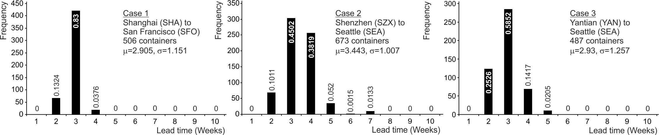
Figure 4.6: PMF of the lead-time in three shipping lanes (Port-to-Port time)

If we had a historical time series of actual shipments, detailing when they were shipped, and when they arrived, we can identify the average lead-time as illustrated in the following example.

Example. Determine \(T_p\) under random lead times. Assuming that the replenishment system operates on a weekly basis, we can use the following procedure to determine the ERP system lead-time, \(T_p\). See also Table 4.2.

• Step 1. Determine the week number of the shipment. This can be done in Excel with the command “=weeknum()”. Care needs to be taken near the year end when the week number gets reset from 52 (or 53 in some years) back to 1.

• Step 2. Determine the week number when that shipment was received using the same procedure as step 1.

• Step 3. Subtract the week number of shipment from the week number of receipt to determine the duration of each shipment.

• Step 4. Find the average lead-time (the average is 3.1).

• Step 5. Round down any non-integer lead time estimates to the nearest integer (i.e. \(T_p=\lfloor 3.1 \rfloor =3).\)

Table 4.2: Determining \(T_p\) when the lead time is random.

Ship date	Week no. shipped	Received date	Week no. received	Lead time in weeks
5 June	24	20 June	26	2
12 June	25	12 July	29	4
19 June	26	28 July	31	5
26 June	27	16 July	29	2
3 July	28	1 August	32	4
10 July	29	1 August	32	3
17 July	30	1 August	32	2
24 July	31	18 August	34	3
31 July	32	24 August	35	3
7 August	33	30 August	36	3
			Average	3.1

4.3 Order-up-to policy

The OUT policy is a popular way to generate production orders in high volume settings. It is a standard policy included in many ERP systems. The OUT policy is especially useful when there is production lead-time present and inventory costs are the most dominant costs to control. The OUT policy is known to be the optimal linear policy (out of all make-to-stock policies that could possibly exist) for controlling inventory.

The order-up-to policy. The OUT policy determines production orders \(q_t\) via the following equation

\[\begin{align} \tag{4.2} q_t=\hat{d}_{t,t+T_p+1}+(f^\star-f_t)+\left(\sum^{T_p}_{i=1}\hat{d}_{t,t+i}-\sum^{T_p}_{i=1}q_{t-i}\right). \end{align}\]

Here

• \(\hat{d}_{t,t+T_p+1}\) is the forecast of the demand, made (and using information only available) at time \(t\), of the demand in the period \(t+T_p+1\). \(T_p\) is the production lead time.
• \(f^\star\) is the FGI safety stock (or target net stock, TNS).
• \(f_t\) is the FGI level at time \(t\).
• \(\sum^{T_p}_{i=1}\hat{d}_{t,t+i}\) is the sum of the forecasted demand over the lead time \(T_p\), this is the target work-in-progress.
• \(\sum^{T_p}_{i=1}q_{t-i}\) is the open production orders at time \(t\), the orders that have been placed, but have not yet been received.

The demand \(d_t\), orders \(q_t\), and inventory \(f_t\) are coupled together via the inventory balance equation. \[\begin{align} \tag{4.3} f_t=f_{t-1}-d_t+q_{t-Tp-1}. \end{align}\]

The OUT policy provides the tightest inventory control possible for a given set of forecasts; the OUT policy is the inventory cost optimal policy. However, more accurate forecasts over the lead time and review period will lead to less inventory requirements.

Table 4.3 illustrates how the OUT determines the production quantity in each period. See if you can build a simple spreadsheet that replicates the numbers in Table 4.3 using (4.2) and (4.3). It will really help to make your understanding of the OUT policy concrete. Note, the variance of the inventory is \(\sigma^2_f=27.44\) and the variance of the production targets \(\sigma^2_q=33.90\).

Table 4.3: Calculating OUT production orders (Notes: \(T_p=1\), \(\alpha=0.5\), \(f^\star=8\))

Time, \(t\)	Demand, \(d_t\)	One period ahead forecast, \(\hat{d}_{t+1|t}\)	Two periods ahead forecast, \(\hat{d}_{t+2|t}\)	Net stock, \(f_t\)	Orders, \(q_t\)
-1	10	10.00	10.00	8.00	10.00
0	10	10.00	10.00	8.00	10.00
1	16	13.00	13.00	2.00	22.00
2	9	11.00	11.00	3.00	5.00
3	8	9.50	9.50	17.00	5.00
4	12	10.75	10.75	10.00	14.50
5	10	10.38	10.38	5.00	9.25
6	14	12.19	12.19	5.50	17.63
7	12	12.09	12.09	2.75	11.81
8	8	10.05	10.05	12.38	3.91
9	10	10.02	10.02	14.19	9.95
10	11	10.51	10.51	7.09	11.98
	\(\sigma^2_d=6.67\)			\(\sigma^2_f=27.44\)	\(\sigma^2_q=33.90\)
				\(NSAmp=4.12\)	\(Bullwhip=5.09\)

4.3.1 Setting the safety stock levels, \(f_t\)

Safety stocks are a target net stock–that we will sometimes be above and sometimes below–that are maintained to ensure availability of product. A common mis-perception is that safety stocks are a minimum level of stock that must always be held. Actually, the minimum stock level is zero; the safety stock, is a target average level, about which the inventory levels will fluctuate. The target safety stock is set so the probability of having no stock, and being unable to satisfy demand immediately, is as low as desired.

The reasons to hold safety stock can be traced to the following sources:

• Demand uncertainty. Demand uncertainty is the un-forecasted component of demand. Recall, the OUT policy (and the POUT policy) attempts to forecast future demand; the forecast errors end up in the inventory levels.
• Supply uncertainty. This can result from either stochastic lead-times, unreliable suppliers, or from supply chain failures (strikes, natural disasters, wars etc.).
• Process uncertainty. Some production technologies are inherently uncertain. For example, we don’t know how many animals or plants will survive the breeding and rearing/growing process. Or the production process is right on the limits of it’s capability and quality, scrap, and rework issues are common. Or the yield of a production process is variable, perhaps because of screening, the use of natural raw materials, or is affected by environmental conditions such as humidity and temperature.

There is plenty of advice for coping with demand uncertainty; we will review some shortly. The standard advice for coping with supply uncertainty is to consider a stochastic lead-time exists and to use some insights about the variance of random sums of random numbers, but the approach is not reliable, often giving incorrect advice. Process uncertainty is usually accounted for by adding in buffer lead-time.

Often the textbook advice is to set the safety stock target as a multiple of the standard deviation of demand multiplied by the lead-time. This is correct when the OUT policy is present, i.i.d. demand is present and the future demand forecasts are set to the mean demand (which is assumed to be known). If you do not know the demand generating process, or the mean demand, or if your forecasting method has not removed all of the signal from the demand process, or you smooth the production orders with the POUT policy, then it is important that you use the standard deviation of the actual net stock levels to set your safety stock.

There are four basic approaches to setting safety stock targets:

1. Use the standard safety stock formula.
2. Simulate the replenishment policy in a spreadsheet.
3. Using judgement and experience.
4. Using NSAmp theory.

Let’s consider each in turn.

The safety stock formula. If your inventory levels (net stock levels) are normally distributed then the target safety stock is given by the following formula:

\[\begin{align} f^\star=z_f \sqrt{L \sigma^2_d}, \end{align}\]

where \(z_f\) is the standard normal variant set to ensure a strategic levels of inventory availability (expressed as a fraction between 0 and 1, rather than as a percentage), \(z_f=\Phi^{-1}[\text{Availability}]\), and \(\Phi^{-1}[\cdot]\) is the inverse of the cumulative distribution function for the standard normal distribution. For 99% availability, \(z_f = \Phi^{-1}[0.99] = 2.32635\), for 95% availability \(z_f = \Phi^{-1}[0.95] = 1.64485\), and for 90% availability \(z_f= \Phi^{-1}[0.90] = 1.28155\).

A Shiny App is available here where we can explore the standard normal distribution interactively. The App can calculate the PDF, CDF and Loss function and their inverses for the standard normal distribution.

To use the standard formula for the safety stock requires us to know the variance of the Net Stock levels. We would usually obtain this from the Net Stock time series, but this information is not actively archived in many companies. It can however be inferred from the inventory balance equation, (4.3). If you try to determine the variance (standard deviation) of the net stock levels from inventory information directly, part of the inventory variability may have been caused by the changing safety stocks in the past (it is important that you determine the variance of the net stock levels during periods when the safety stock has remained constant). The use of the inventory balance equation often allows you to untangle the impact of any changing safety stock targets. Table 4.4 details the calculation required to determine the computed inventory levels, and then determine the variance of the inventory levels.

Table 4.4: Determining the variance of the inventory levels via the inventory balance equation¹⁴

Time, \(t\)	Completions, \(q_{t-T_p-1}\)	Demand, \(d_t\)	Computed net stock, \(f_t=f_{t-1}+q_{t-T_p-1}-d_t\)	Variance calculation \((f_t-\mu_f)^2\)
0	-	-	8	-
1	8	10	6	1
2	4	6	2	9
3	12	8	6	1
4	10	12	4	1
5	13	10	10	25
6	8	14	6	1
7	7	12	4	1
8	9	8	6	1
9	6	10	2	9
10	12	10	4	1
		Average	\(\mu_f=5\)	\(\sigma_f^2=5\)

First, we select an initial opening stock and then, in the fourth column, we determine the computed net stock via the inventory balance equation. After we reach time 10, we average the computed net stock in periods 1 through 10, \(\mu_f = 5\). Then we calculate the fifth column, the squared difference of the computed net stock and the average computed net stock. Finally, the variance is the average of these squared differences, \(\sigma^2_f = 5\).

Note: The initial inventory level can be set by either; referring to a stock count report from the past, or via trial and error in an Excel simulation you can determine the initial inventory level required to ensure the final inventory matches your current inventory. Either way, the initial inventory choose does not affect the final variance calculation, the inventory variance will always equal five in this example.

The safety stock formula is useful, but it takes no account of supply or process uncertainty. If you used the variance of the net stock (rather than the often recommended \(f^\star=z \sqrt{L\sigma^2_d}\)) then you are also properly accounting for the requirements for inventory generated by the smoothing in the POUT policy.

Simulate the replenishment policy in a spreadsheet. This approach has the advantage of being able to use real demand. You can also simulate the consequences of supply and process uncertainties as well as the influence of stochastic lead-times.

Using judgement and experience. You may be aware that certain raw materials are only available from a single supplier, or perhaps a limited number of suppliers, due to intellectual property or technical issues. Or perhaps some raw materials have a long lead-time, are only available during certain times of the year, or have very large minimum order quantity. For these products, you may wish to abandon all safety stock formulas and decide to hold a large strategic raw material inventory to minimise the risk of not having adequate supplies.

Safety stocks should be kept constant, for perhaps a quarter, before being reviewed and adjusted to reflect the most recent data. If you adjust your safety stocks too frequently then, as the change in the safety stock will be passed directly to production, the safety stock adjustments themselves will introduce variability into the system. It may be possible to spread out the change in safety stock over several planning periods.

Setting safety stocks to minimise inventory holding and backlog costs. Consider the following per unit inventory holding and backlog costs are incurred each time period:

\[\begin{align} \tag{4.4} \text{Inventory costs, }C_{i,t}=h [f_t]^+ +b[-f_t]^+, \end{align}\]

Unit inventory holding costs are usually determined as a percentage of the cost (material purchase cost and any added value plus an allowance for storage, insurance, obsolescence, and capital costs). There are two approaches to set backlog costs. Either, the net present value of all future forgone cash flows resulting from a backlog is used. Or, a pseudo backlog cost is specified to ensure the optimal safety stock identified later achieves a strategic level of inventory availability.

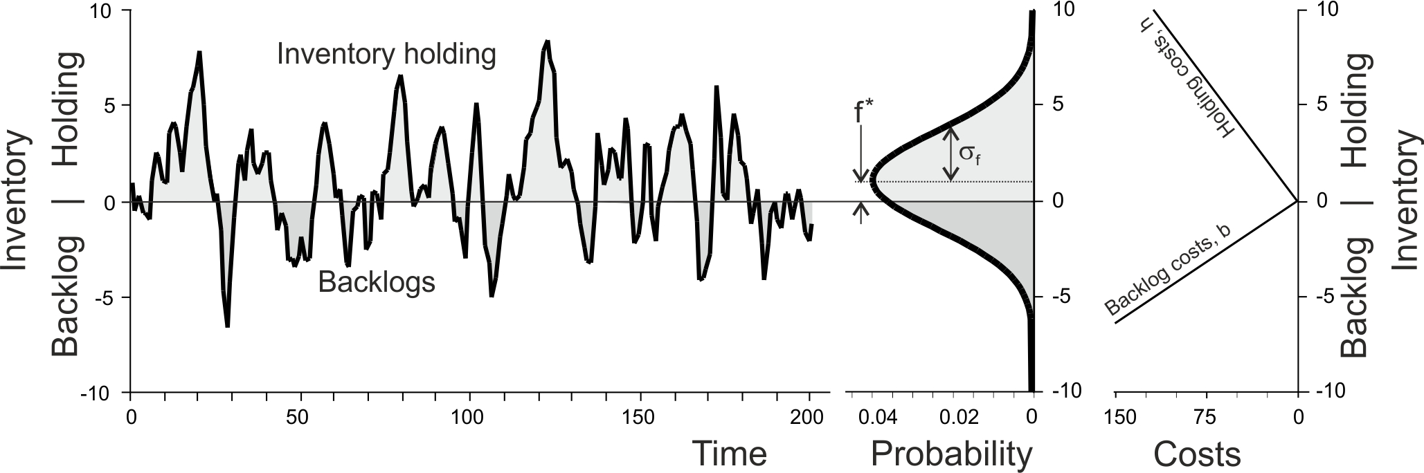
Figure 4.7: Inventory holding an backlog costs over time

Under normally distributed (but possibly correlated) demand, it can be shown, using standard newsvendor techniques that the inventory holding and backlog costs are minimised by setting the safety stock, \(f^\star\) equal to

\[\begin{align} \tag{4.5} f^\star=\sigma_{f} z_f: z_f=\Phi^{-1}\left[\frac{b}{b+h}\right]. \end{align}\]

Here, \(\sigma_f\) is the standard deviation of the FGI levels. If the auto-covariance structure of the demand process, the forecasting mechanism and the production lead time is known, it is possible to find a closed form NSAmp expression that can be used in the safety stock calculation. Using the NSAmp ratio also has the advantage as structural insight can be gained, providing direction to company executives.

The resulting minimum inventory holding costs, when a safety stock of \(f^\star\) is present, is given by \[\begin{align} \tag{4.6} C_f^\star=\sigma_{f}(b+h)\phi[z_f]. \end{align}\] Notice, (4.6) is a linear function of the standard deviation of the inventory, \(\sigma_f\). Thus, the more variable the inventory, the more safety stock is required and the more inventory holding and backlog costs are incurred.

To use (4.5) to set safety stock levels we need to know \(\sigma_f\). We can obtain this from the NSAmp ratio, which in turn depends on the demand process, the forecasting mechanism, and the lead time. We will explore this in more detail in Section 4.3.3. However, before the do that we will first explore two ways to determine the optimal capacity levels required in our production system.

4.3.2 Optimal capacity levels

Another question that we need to answer with the OUT policy is how much production capacity do we need? It depends on your cost structure and context; here we review two scenarios. One scenario has production costs dominated by capital investment (for example, in highly automated capital intensive settings). The other scenario is relevant when the production capacity costs are dominated by labour costs.

OUT capacity levels to minimise opportunity loss and overtime costs

Per period capacity costs \(C_{q,t}\) are incurred as follows,

\[\begin{align} \tag{4.7} C_{q,t}=n (k+\mu_d-q_t)^+ +p (q_t-k-\mu_d)^+. \end{align}\]

Here, \(n\) is the opportunity loss incurred for each unit of unused capacity and \(p\) is a per unit cost to produce items in over-time, above the nominal capacity of \(\mu_d+k\), where \(\mu_d\) is the mean demand and \(k\) is the slack capacity. \(k\) can be both positive and negative. The cost function in (4.7) may be suitable in highly automated, capital intensive, settings.

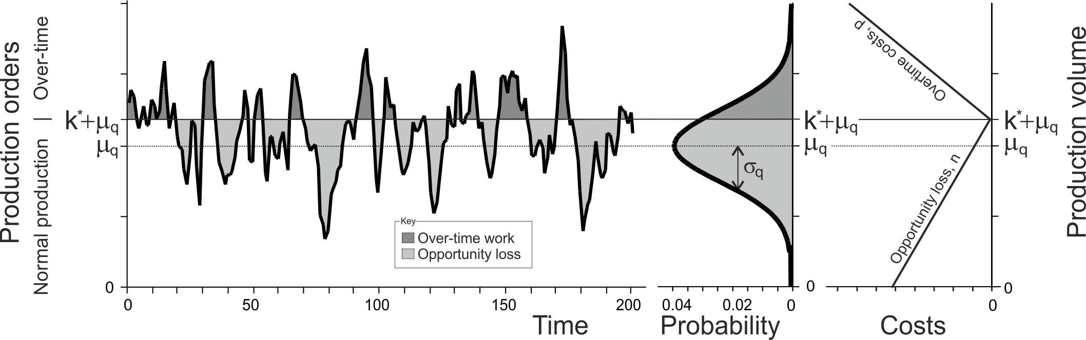
Figure 4.8: Opportunity loss and over-time costs over time

The expected capacity costs \(\mathbb{E}[C_{q,t}]\) are minimised when the nominal capacity level is set to \(\mu_d+k^\star\) where,

\[\begin{align} \tag{4.8} k^\star=\sigma_q z_q; \quad z_q=\Phi^{-1}\left[\frac{p}{p+n}\right]. \end{align}\]

The minimised opportunity loss and overtime costs \(C^\star_q\) are given by,

\[\begin{align} \tag{4.9} C^\star_q=\sigma_q(n+p)\phi[z_q] \end{align}\]

Capacity costs are convex in \(k\), thus \(k^\star\) is a global minimum. Notice, the minimised capacity costs are linearly related to the standard deviation of the production orders, \(\sigma_q\). Again, this depends on the demand process, the forecasting mechanism, and lead times. We will explore these factors further in Section 4.3.3.

OUT capacity levels to minimise guaranteed hours and overtime costs

Assume we have an installed production capacity of \(\tilde{k}\). Each unit produced by the installed capacity in normal working hours costs \(u\) monetary units. If the production requirements are less than \(\tilde{k}\), the production capacity (labour) stands idle for part of the week, but the we still pay \(u\tilde{k}\) (that is, we still pay a regular weekly wage to our staff). However, if we need to produce more than our weekly capacity (more than \(\tilde{k}\) units) we can run overtime on the weekend to make up the shortfall at unit overtime cost \(w\), where \(w>u\). These costs can be represented by

\[\begin{align} \tag{4.10} \text{Capacity costs, }\tilde{C}_{q,t}=u\tilde{k}+w[q_t-\tilde{k}]^+. \end{align}\]

This cost function may be most suitable in settings dominated by labour costs. Notice that the overtime quantity is flexible; staff only work to produce \([q_t-\tilde{k}]^+\) items in overtime, which maybe less than a full shift of work. Figure 4.9 illustrates the installed capacity and overtime costs.

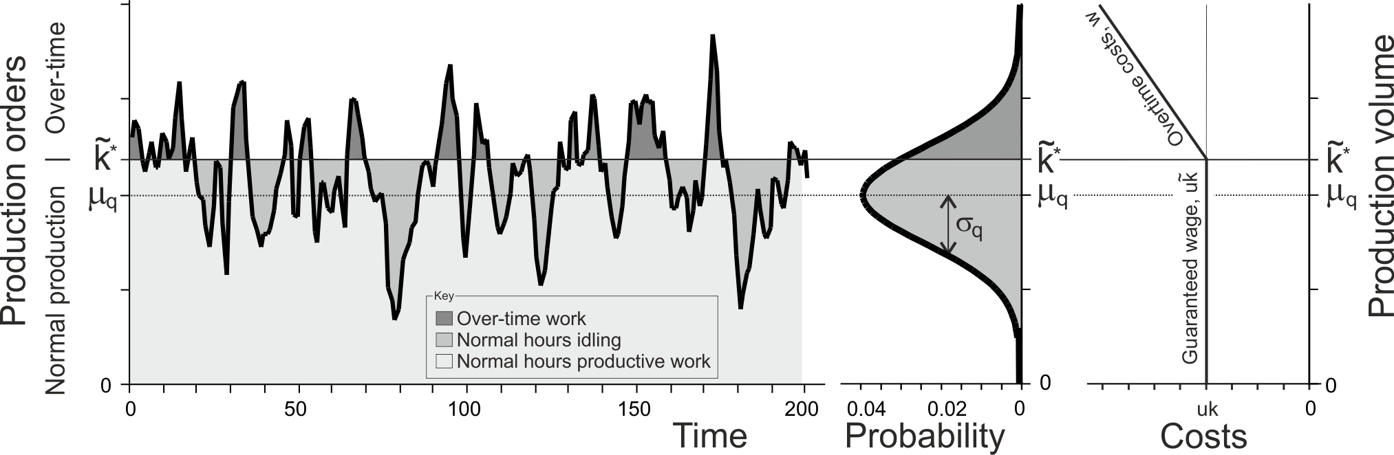
Figure 4.9: Over-time and idling capacity costs with guarenteed labour hours over time

There happens to be an optimal capacity level \(\tilde{k}^\star\) to install that minimises the expected per period capacity costs, \[\begin{align} \tag{4.11} \tilde{k}^\star=\mu_d+\tilde{z}_q \sigma_q: \tilde{z}_q=\Phi^{-1}\left[\frac{w-u}{w}\right]. \end{align}\] When an optimal capacity level is present, \(\tilde{k}=\tilde{k}^\star\), the minimised expected capacity will then be \[\begin{align} \tag{4.12} \tilde{C}^\star_q=\mu_d u +w \sigma_q \phi[\tilde{z}_q]. \end{align}\]

We see that the minimised expected capacity costs, \(\tilde{C}^\star_q\) is a linear function of the standard deviation of the production rate \(\sigma_q\), offset by a constant \(\mu u\). We also know that there is a minimum unique \(\tilde{k}^\star\) as the total capacity costs is convex in \(\tilde{k}^\star\).

4.3.3 Bullwhip and NSAmp in the OUT policy

The order-up-to policy requires forecasts of future demand when calculating the production targets. This forecasts will have an influence on the Bullwhip and NSAmp ratios, the safety stock and capacity requirements, and the inventory and capacity costs. While the Bullwhip and NSAmp ratio will depend on the auto-correlation structure of the demand process, for some special cases we have been able to obtain closed form expressions for these ratios. These are important as they give us some structural insight on the parameters of the forecasting system, and the lead time, on the dynamic and economic behaviour of the system. The simplest random demand structure is the independently and identically distributed (i.i.d.) demand process, an uncorrelated random demand process. Next, we will review a number variance ratios maintained by the OUT policy under i.i.d. demand. Note, the variance ratios hold regardless of the distribution of the demand (they are distribution free), but the remarks we make about the economics of the OUT policy require the demand to be normally distributed.

Naïve forecasts There are no parameters in the Naïve forecasting mechanism, but both the Bullwhip and the NSAmp ratios (for i.i.d. demand) reveal the standard deviation of the orders and the FGI levels are increasing in the lead time \(T_p\) as the Bullwhip ratio \[\begin{align} \tag{4.13} \text{Bullwhip = }\frac{\sigma^2_q}{\sigma^2_d}=2(1+2T_p+T_p^2), \end{align}\] is a quadratic function of \(T_p\). The NSAmp ratio is also a quadratic function of \(T_p\), \[\begin{align} \tag{4.14} \text{NSAmp = }\frac{\sigma^2_f}{\sigma^2_d}=2+3T_p+T_p^2. \end{align}\] Both the Bullwhip and NSAmp expressions are also always greater than two, even with \(T_p=0\). This indicates that the orders and FGI will be at least twice as variable as the demand.

Exponential smoothing forecasts Under i.i.d. demand, Dejonckheere et al. (2003) show the OUT policy with exponential smoothing forecasts has a Bullwhip ratio of

\[\begin{align} \tag{4.15} \text{Bullwhip}=\frac{\sigma^2_q}{\sigma^2_d}=1+2\alpha(T_p+1)+\frac{2 \alpha^2(T_p+1)^2}{2-\alpha} \end{align}\]

When \(\alpha\rightarrow 0\), the Bullwhip ratio approaches a minimum of unity; the standard deviation of the orders will also be minimised when \(\alpha\rightarrow 0\) (and so will be the optimal capacity \(k^\star\) and the capacity costs). The production orders are always more variable than demand, \(\sigma^2_q\geq \sigma^2_d\). Thus, we can see that as we make more accurate forecasts the Bullwhip problem is reduced (but is not eliminated in the OUT policy with exponential smoothing forecasts. When \(\alpha=1\), the Bullwhip maintained by the OUT policy with exponential smoothing forecasts equals the Bullwhip maintained by the OUT policy with Naïve forecasts. Finally, we can also see the value of lead time reduction in (4.15). Shorter lead times always reduce the Bullwhip effect and the order variance (hence, the capacity requirements \(k^\star\), and the capacity costs (\(C^\star_q\) and \(\tilde{C}^\star_q\)) will also be reduced). Figure 4.10 plots the Bullwhip generated by the OUT policy with exponential smoothing forecasts for different lead times.

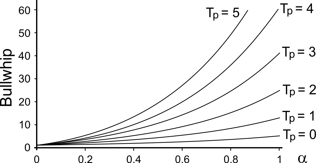
Figure 4.10: Bullwhip generated by the OUT policy with exponential smoothing forecasts under i.i.d. demand

The NSAmp ratio maintained by the OUT policy with exponential smoothing forecasts under i.i.d. demand is given by

\[\begin{align} \tag{4.16} \text{NSAmp}=\frac{\sigma^2_f}{\sigma^2_d}=1+T_p+\frac{\alpha(1+T_p)^2}{2-\alpha}. \end{align}\]

The NSAmp ratio is always larger than \(1+T_p\). The minimum NSAmp (\(=1+T_p\)) occurs when \(\alpha=0\). NSAmp is increasing convex in both \(\alpha\) and \(T_p\). NSAmp is a quadratic function of the lead time \(T_p\). Equation (4.16) reveals that there is an inventory benefit to reducing the lead time \(T_p\). When \(\alpha=1\), the NSAmp produced by the OUT policy with exponential smoothing forecasts matches the NSAmp maintained by the OUT policy with Naïve forecasts. Figure 4.11 plots the NSAmp generated by the OUT policy with exponential smoothing forecasts for different lead times.

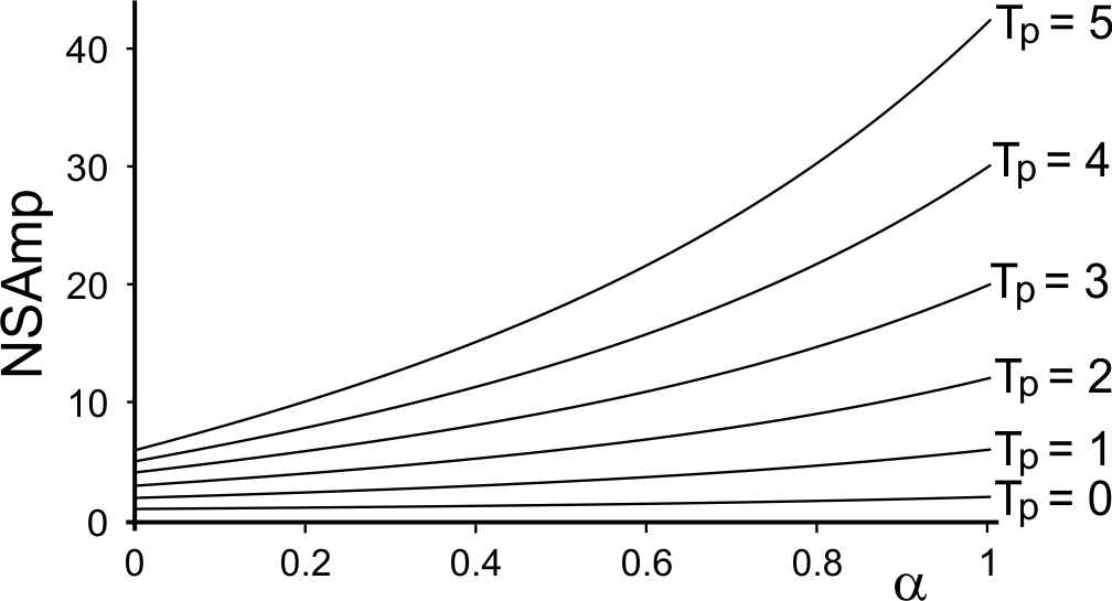
Figure 4.11: The NSAmp maintained by the OUT policy with exponential smoothing forecasts under i.i.d. demand

Moving average forecasts The Bullwhip effect produced by the OUT policy with moving average forecasts under i.i.d. demand is described in (4.17) \[\begin{align} \tag{4.17} \text{Bullwhip}=\frac{\sigma^2_q}{\sigma^2_d}=1+\frac{2(T_p+1)}{m}+\frac{2 \alpha^2(T_p+1)^2}{m} \end{align}\] Bullwhip in decreasing in \(m\), the number of periods of data used in the moving average forecast. As \(m\rightarrow \infty\), then the Bullwhip ratio approaches unity, but as always \(\sigma^2_q\geq \sigma^2_q\), Bullwhip is always present. Furthermore, the Bullwhip ratio also always increases in the lead time \(T_p\).

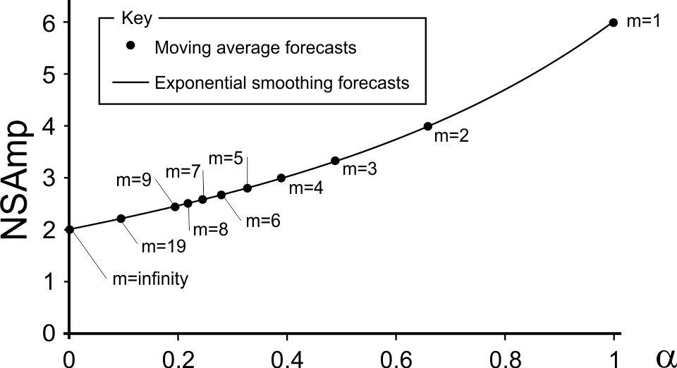
Figure 4.12: The Bullwhip maintained by the OUT policy with moving average forecasts under i.i.d. demand when \(T_p=1\)

The NSAmp maintained by the OUT policy with moving average demands under i.i.d. demand is given by \[\begin{align} \tag{4.18} \text{NSAmp}=\frac{\sigma^2_f}{\sigma^2_d}=\frac{(T_p+1)(T_p+1+m)^2}{m} \end{align}\] Equation (4.18) is decreasing in \(m\) and increasing in \(T_p\). As \(m\rightarrow\infty\) the moving average forecasts approach the MMSE forecast (of the mean demand, assuming it is known) and the OUT-MA policy minimises the variance of the FGI levels (to the minimum of \(\sigma_f^2=\sigma_d^2(1+T_p)\)).

Figure 4.13 illustrates the NSAmp of the OUT-MA policy under i.i.d. demand. We have plotted the exponential smoothing \(\alpha\) on the x-axis for comparison. As \(m\) is an integer greater than zero, \(m\in\mathbb{N}_+\), the OUT-MA NSAmp can only be compared to the OUT-ES NSAmp at specific \(\alpha\) points (shown with the dots). The dots have been place on x-axis where the average of the data in moving average forecast \((m-1)/2\) equals the average age of the data in the exponential smoothing forecast \(1/\alpha-1\). At those points, the OUT-MA NSAmp concurs with the OUT-ES NSAmp. This relationship holds for all lead times; this insight, together with Figure 4.11 makes it easy to visualise/understand the impact of the lead time \(T_p\) on the OUT-MA policies NSAmp metric.

Figure 4.13: The NSAmp maintained by the OUT policy with moving average forecasts under i.i.d. demand when \(T_p=1\)

**** Add some example calculations for determining the \(f^\star\), \(k^\star\) and the minimised total costs for each of the forecasting methods, for different lead times. Use it to illustrate the value of lead time reduction. ****

It is known that the OUT policy with naïve, moving average, exponential smoothing, and Holt’s method forecasts all produce the bullwhip effect, for all lead times, and all demand processes (not just i.i.d.), see Dejonckheere et al. (2003) and Li, Disney, and Gaalman (2014). However, the OUT policy with damped trend forecasts does not always produce bullwhip if some particular parameter settings are used, Li, Gaalman, and Disney (2023). One is left wondering is there a way to avoid bullwhip with the simpler forecasting method? Yes, there is. It is called the proportional order-up-to policy. We study this in the next section.

4.4 Proportional order-up-to policy

The proportional order-up-to (POUT) policy

The POUT policy generates production orders \(q_t\) via, \[\begin{align} q_t=\hat{d}_{t,t+T_p+1}+\frac{1}{T_i}\left(f^\star-f_t\right)+\frac{1}{T_i}\left(\sum^{T_p}_{i=1}(\hat{d}_{t,t+i}-q_{t-i})\right) \end{align}\]

As with the OUT policy:

• \(q_t\) is the production/distribution order made at time \(t\).
• \(\hat{d}_{t,t+T_p+1}\) is the forecast of the demand, made (and using information only available) at time \(t\), of the demand in the period \(t+T_p+1\).
• \(f^\star\), is a safety stock to ensure adequate inventory service levels.
• \(f_t\) is the net stock at time \(t\). If \(f_t>0\), then inventory is available, if \(f_t<0\) a backlog exists (in some situations the negative inventory is not allowed as sales are lost when there is no inventory to satisfy demand, in which case \((f_t<0)^+\) may be used instead).
• The sum of demand over the lead-time \(\sum_{i=1}^{T_p}\hat{d}_{t,t+i}\) is the desired work-in-process (a.k.a. the desire in-transit inventory).
• \(\sum_{i=1}^{T_p} q_{t-i}\) are the actaul WIP, the open orders, the orders placed but not yet received.

The POUT policy also contains the feedback parameter, \(1/T_i\), which regulates the speed at which deviations between the safety stock and actual inventory are corrected; \(1/T_i\) also regulates how fast deviations from the target WIP and actual WIP are corrected. \(0\leq 1/T_i<2\) is required for stability.

The inventory balance equation, (4.3), completes the POUT policy.

Note, negative production orders may happen if there is a large negative demand or if the orders have a high variance in relation to its mean (this should be a relatively rare occurrence). A negative \(q_t\) means that some FGI needs to be disassembled into raw materials. In some cases this is not possible (it is not possible to disassemble an omelette for example) or not economic. Then the orders can be truncated to be non-negative, i.e. \((q_t)^+\), and a negative production order is replaced with a zero production order.

Example calculation of the POUT replenishment decision. Let’s illustrate the calculation of the POUT policy replenishment decision by way of a numerical example. Consider here the lead-time \(T_p=1\), the safety stock is \(f^\star=8\) and the demand, one period ahead, and two period ahead forecasts are as detailed in Table 3.7. **** Need to update Table 3.7 with this new demand pattern ****

Make a comparison with Table 4.3*

Table 4.5: Calculating POUT production orders¹⁵ (\(T_p=1\), \(\alpha=0.5\), \(f^\star=8\), \(T_i=8\))

Time, \(t\)	Demand, \(d_t\)	One period ahead forecast, \(\hat{d}_{t+1|t}\)	Two periods ahead forecast, \(\hat{d}_{t+2|t}\)	Net stock, \(f_t\)	Orders, \(q_t\)
-1	10	10.00	10.00	8.00	10.00
0	10	10.00	10.00	8.00	10.00
1	16	13.00	13.00	2.00	14.13
2	9	11.00	11.00	3.00	11.23
3	8	9.50	9.50	9.13	9.14
4	12	10.75	10.75	8.36	10.91
5	10	10.38	10.38	7.50	10.37
6	14	12.19	12.19	4.41	12.86
7	12	12.09	10.09	2.78	12.65
8	8	10.05	10.05	7.64	9.77
9	10	10.02	10.02	10.29	9.77
10	11	10.51	10.51	9.06	10.47
	\(\sigma^2_d=6.67\)			\(\sigma^2_f =9.36\)	\(\sigma^2_q=2.56\)
				\(NSAmp=1.40\)	\(Bullwhip=0.38\)

Notice, the same demand, forecasts, lead-time, and safety stock are used in Table 4.5 as was used in Table 4.3 for the OUT policy. The OUT policy produced an \(NSAmp=4.12\) and \(Bullwhip=5.09\). However, the POUT policy with a feedback controller of \(T_i=8\) reduced the variance ratios to \(NSAmp=1.40\) and \(Bullwhip=0.38\). Amazing huh?

4.4.1 The inventory and order variance trade-off: The POUT policy under i.i.d demand with MMSE forecasts

Suppose demand was an independently and identically distributed (i.i.d.) random variable with a constant mean and constant variance. As there is no demand autocorrelation, the best possible forecast from an inventory viewpoint (as minimum mean squared error forecasts are produced for all future demands) is to set all future forecasts equal to the mean demand. This is also the best possible forecast from bullwhip viewpoint (as the variance of the forecasts is zero). MMSE forecasts of i.i.d. demand can be created by setting the first forecast to the mean demand and using \(\alpha=0\) in the exponential smoothing forecasting method.

Variance ratios for the POUT policy with i.i.d. demand and MMSE forecasts

The variance of the production orders issued by the POUT policy is given by \[\begin{align} \tag{4.19} \mathbb{V}[o_t]=\mathbb{V}[d_t]\left(\frac{1}{2T_i-1}\right) \end{align}\] which is increasing in \(1/T_i\). The FGI variance maintained by the POUT is convex in \(1/T_i\) with a minimum at \(T_i=1\) and is given by \[\begin{align} \tag{4.20} \mathbb{V}[f_t]= \mathbb{V}[d_t]\left( 1+T_p+\frac{(T_i-1)^2}{2 T_i-1}\right). \end{align}\] Note: For a stable system the valid range of \(T_i\) is \(0.5<T_i<\infty\).

Notice, as \(0.5<T_i<\infty\), then \((T_i-1)^2/(2 T_i-1)>0\), and the inventory variance is always larger than the demand variance. The variance of the FGI also increases in the production lead time \(T_p\). The consequences of this, in a practical setting, is that reducing the production lead time leads to reduced inventory variance (and hence smaller safety stock requirements).

Also notice, from Figure 4.14,that if we are using the POUT policy to smooth demand then we are basically accepting a higher inventory variability in return for smoother production orders. However, we are fortunate as we can buy a lot of production smoothing with relatively little extra inventory variability, as the inventory variance has a fairly shallow basin near the inventory variance minimum at \(T_i=1\).

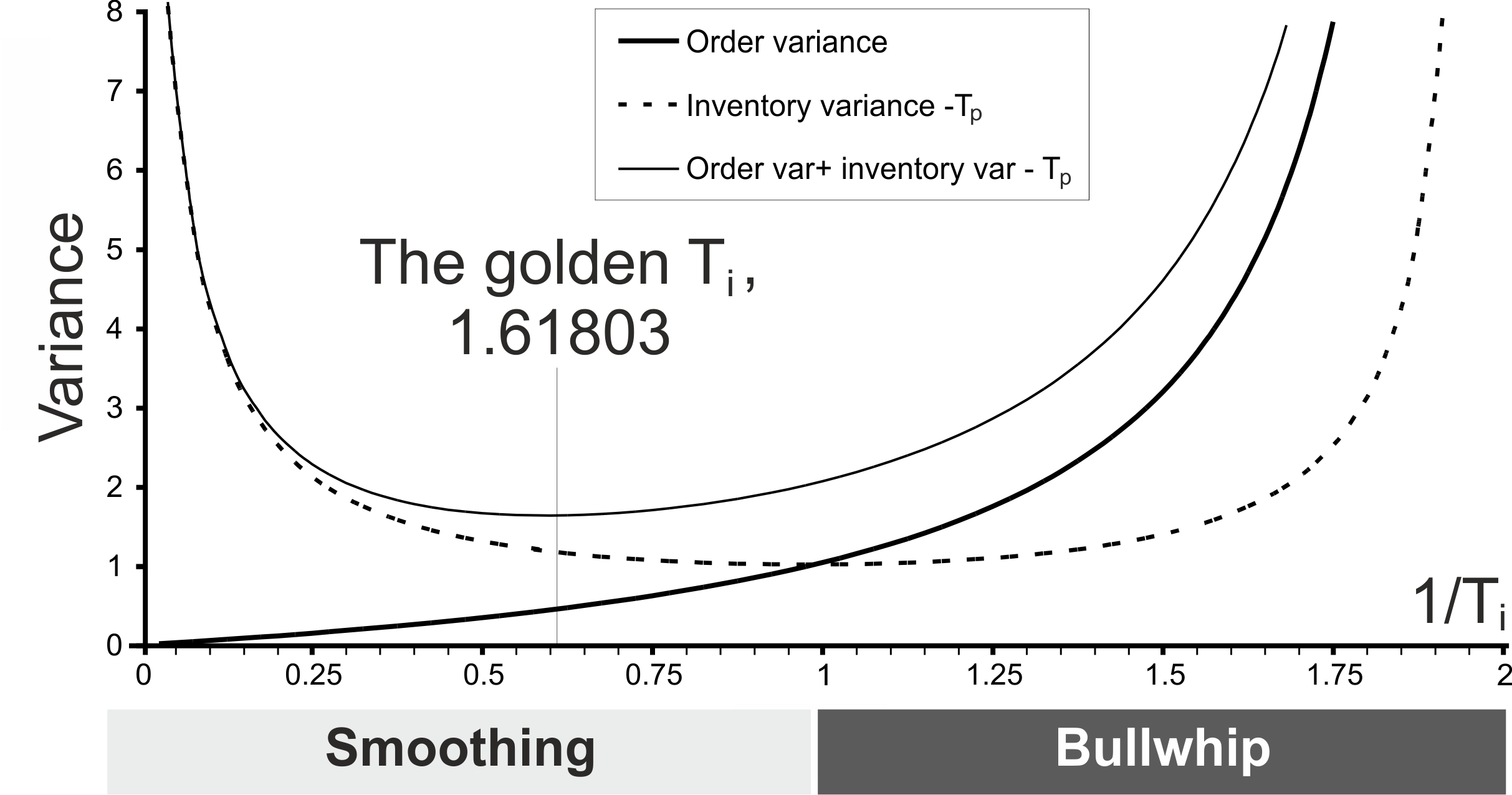
Figure 4.14: The inventory and order variance trade-off (Note, with unit demand variance this also illustrates the Bullwhip and NSAmp ratios)

Figure 4.14 also plots the sum of inventory and order variance (with unit demand variance). This objective function has an intriguing solution.

The golden ratio solution

We may be interested in minimising the sum of the production variance and the finished goods inventory variance. Adding the two variances together produces a convex total variance curve with a minimum at \(T_i=(1+\sqrt{5})/2 =1.618034\), the golden ratio. See Figure 4.14. We can prove this fact with a little bit of calculus. First we create an objective function \(J\), \[\begin{align} \tag{4.21} J=Bullwhip+NSAmp=\frac{1}{2T_i-1}+1+T_p+\frac{(T_i-1)^2}{2T_i-1}. \end{align}\] Then we differentiate \(J\) with respect to \(T_i\), \[\begin{align} \tag{4.22} \frac{dJ}{dT_i}=-\frac{2}{(1-2T_i)^2}+\frac{2T_i(1-T_i)^2}{(1-2T_i)^2}=\frac{1}{2}-\frac{5}{2(1-2T_i)^2}. \end{align}\] Solving \(dJ/dT_i=0\) for \(T_i\) yields \[\begin{align} \tag{4.23} \frac{1}{2}=\frac{5}{2(1-2T_i)^2}\implies T_i=\frac{1\pm\sqrt{5}}{2}=\{-0.618034,1.618034\}. \end{align}\] Discarding the negative \(T_i\) (as it is outside of the stability region and is not valid) implies \(T_i=1.618034\), the so-called golden ratio.

Although the golden ratio is an elegant solution (this beautiful number can be found throughout nature, maths, and art), unfortunately it this is not the minimum cost solution. In order to find that we need to quantify minimum possible inventory and capacity costs. Those costs require us to set the safety stock \(f^\star\) and capacity levels to certain optimum levels which themselves are a function of the feedback parameter, \(T_i\).

4.4.2 Economics of the POUT policy

Suppose that we incur inventory holding and backlog costs as given by (4.4). These costs are minimised by setting \(f^\star\) equal to (4.5); the resulting minimised inventory costs will then be given by (4.6). The POUT policy incurs inventory holding and backlog costs in the exact same way as the OUT policy, the only difference is that the standard deviation of the inventory levels maintained by the POUT is is different to the standard deviation of the inventory levels maintained by the OUT policy (recall it is known that, in the long run, the OUT policy will always have less inventory variability than the POUT policy as the OUT is the optimal policy for reducing inventory costs).

We can also apply the OUT capacity cost functions to the POUT policy. For example, if we incurred capacity costs as defined by (4.7) (or (4.10)), setting our nominal capacity level to (4.8) (or (4.11)) results in minimised opportunity loss and overtime costs (or minimised guaranteed wages and overtime). This minimised capacity costs are given by (4.9) (or (4.12)).

Notice, both (4.9) and (4.12) are linear functions of the standard deviation of the production orders, \(\sigma_q\). The POUT policy is able to reduce the standard deviation of the orders by setting the proportional feedback controller \(T_i\), see Figure 4.14. All that remains now is to optimise the feedback controller \(T_i>1.\)

4.4.3 Tuning the feedback controller \(T_i\) to minimise the sum of inventory and capacity costs.

Let us first consider an objective function Adding together (4.6) and ref(eq:capOptCosts) creates a total cost function, \[\begin{align} \tag{4.24} TC=\sigma_f(h+b)\phi[z_f]+w\sigma_q\phi[z_q]+u\mu \end{align}\] which is valid when both the safety stock \(f^\star\) and the optimal capacity level \(\tilde{k}^\star\) is present. Both \(f^\star\) and \(\tilde{k}^\star\) depend upon the optimal feedback parameter \(T_i^\star\), which we have yet to determine. We do that now, first for the case when \(T_p=0\), where for i.i.d. demand with MMSE forecasts, we are able to gain an analytical solution. For non i.i.d. demand (correlated demands), non-MMSE forecasts, and/or lead times \(T_p>0\), we have to resort to numerical search techniques.

The economic feedback parameter, \(T_i^\star\).

The total cost function (4.24) can be written as \[\begin{align} \tag{4.25} TC=\varphi(\sigma_f+\lambda(\sigma_q-\sigma_f))+u\mu \end{align}\] where \(\varphi=(h+b)\phi[z_f]+w\phi[z_q]\) is a scaling factor, \(\lambda=w\phi[z_q]/\varphi\) is a capacity intensity factor. The \(u\mu\) term, is independent of \(T_i\) and will disappear under differentiation. Substituting in \(1/T_i=(1-\tau)\), and differentiating TC with respect to \(\tau\) provides \[\begin{align} \tag{4.26} \frac{dTC}{d\alpha}=\varphi\left(\frac{(1-\lambda)\frac{d\sigma^2_f}{d \tau}}{2 \sigma_f}+\frac{\lambda\frac{d \sigma^2_q}{d \tau}}{2 \sigma_q}\right) \end{align}\] The first order condition for the optimal \(\tau^\star\) is \[\begin{align} \tag{4.27} \frac{(1-\lambda)\frac{d\sigma^2_f}{d \tau}}{2 \sigma_f}=\frac{\lambda\frac{d \sigma^2_q}{d \tau}}{2 \sigma_q} \end{align}\] Rearranging (4.27) for \(\lambda\) provides the following inverse function for \(\tau^\star\), \[\begin{align} \tag{4.28} f[\tau]=\frac{\sigma_q}{\sigma_q-\sigma_i\left(\frac{d\sigma^2_f}{d \tau}\bigg{/} \frac{d\sigma^2_i}{d \tau}\right)} \end{align}\] For a given capacity intensity \(\lambda\in[0,1]\), the optimal smoothing parameter is given by \(\tau^\star=f^{-1}[\lambda]\). Sometimes this inverse function can solved analytically (for i.i.d. demand, \(\tau^\star=\lambda\) which implies \(T_i^\star=(1-\tau^\star)^{-1}=(1-\lambda)^{-1}\)), but it is always easily solved graphically or numerically as there is only one \(\tau\) for the optimal \(\lambda\). This allows the regula falsi method (also known as the method of false position) to be used to search for optimal solutions, Boute et al. (2022).

The solution for for i.i.d. demand, \(\tau^\star=\lambda \implies T_i^\star=(1-\tau^\star)^{-1}\), reveals that when labour is more rigid, capacity becomes more constrained and you should smooth more, exactly because it reduces production variance.

Table 4.6: Proportional order-up-to policy implementation methods

Implementation method	Advantages	Disadvantages
Custom coding user defined macros in your ERP systems’ planning book	Allows you to automate the process: minimizes manual data input, consistent set of data. Scalable. Can be applied to many thousands of products.	Requires competency at coding within ERP systems. Data and supply chain settings can be changed by many different people in the organization. Do they all appreciate the consequences of the changes they make?
Custom coding bespoke IT systems	Very flexible approach. Presumably your company has the IT skills to code its own bespoke IT system.	Lack of support from either the software vendor or the user community.
Developing Excel-based decision support systems.	Low initial development costs.	Extra manual data input. Multiple records are held, leading to opportunities for errors and inconsistency.

4.4.4 Overtime and purchase orders

During periods of high demand, you may be using overtime on the weekend to meet weekly production targets. This could create some issues with the integrity of the data if not handled correctly. For example, assume Sunday 23.59 GMT is the end of one planning period, Monday 00.00 GMT is the start of a new planning period. White collar workers (doing the production planning, transportation, etc.) work 9.00-17.00 Monday through Friday. Overtime might be conducted over the weekend and products not shipped to customers until Monday when the logistics team next comes back to the office. If the weekend production is assigned to inventory in the following week, then the ERP system will erroneously count it as inventory and reduce the production orders in the next order calculation. The weekend production should be allocated to a purchase order (PO) opened in the previous week, and then it will not be counted as inventory; rather it will properly assign last week’s production as goods-in-transit to the customer. Furthermore, unallocated inventory (if weekend production was more than the open PO quantities) will be considered as current inventory and next week’s production will be reduced. If the PO quantities were not met then (if weekend production did not achieve the targets), the unmet demand would also be added to next week’s production. Figure 4.15 illustrates the sequence of events and how purchase orders can be used to coordinate the scheduling, production, and shipping activities.

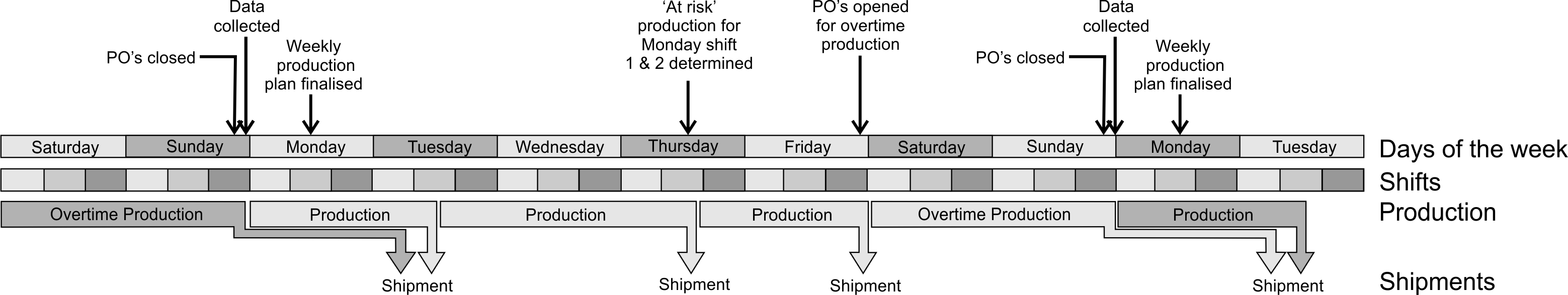
Figure 4.15: Sequence of events during the working week

Notice Figure 4.15 also shows that it is not until the middle of Monday morning that the production plan is finalized. This means that the shift that works 00.00 to 8.00 and 8.00 to 16.00 on Mondays may not be completely scheduled yet. Rather than wasting these production slots, a high demand volume item (or items) should be produced at risk in these shifts. Selecting the high volume items will minimize the chance of over-producing items that are not needed.

4.4.5 Plant shut-downs and maintenance

Suppose that you wish to build ahead for a period of non-production (holiday, maintenance, etc.). This can be managed with independently planned requirements (IPR). First, you need to make a forecast of demand over the shut-down period. If this pre-build can be produced in the last period before the shut-down, then you simply add the additional forecasted demand to the last order before the shut-down as an IPR. Upon returning to work (and after the lead-time), the inventory levels will have returned to normal levels, fluctuating around the safety stock.

However, if you wish to produce the pre-build over several periods preceding the shut-down you will need to add IPR orders over several periods as well as account for the corrective action that the (P)OUT policy will attempt to make to react to what it perceives as an overproduction. This can be done in one of two ways:

1. Adding the accumulated previous IPR’s into the safety stock, i.e. \(f_t=f^\star+\sum_{i>0}IPR_{t-i}\), or

2. Inflating the current week’s IPR to counteract the correction that the (P)OUT will attempt to make by adding \(IPR_t+\sum_{i>0} IPR_{t-i}/T_i\) to the current IPR order.

Both these approaches result in the same dynamic response.

Example: Strategies for pre-building for a shut-down. Suppose that we wanted to pre-build over a period of 4 weeks for a shut-down of 4 weeks. The undisturbed orders are always \(q_t=1, \forall t\), \(T_i=2\) and the normal safety stock, \(q^\star=2\), and the lead-time, \(T_p=2\). Under this demand pattern, we need to pre-build four units of inventory to cover the shut-down period, one unit of IPR in each of the four weeks before the shut-down.

In option (a) we add a unit of production as IPR to the orders in each of the four weeks preceding the shut-down. We also add the accumulated previously issued IPR to the safety stock, creating a dynamic \(TNS_t\). When the shut-down period is over, we reset the IPR back to zero and reset the safety stock levels to the static \(TNS\). Table 4.7 details how option (a) plays out over time in our numerical example.

Table 4.7: Establishing a pre-build to a shut down with IPR and safety stock adjustments

Time, \(t\)	Order, \(q_t\)	IPR, \(IPR_t\)	TNS, \(f^\star_t\)	Adjusted order, \(\tilde{q}_t=O_t+IPR_t\)	Net Stock, \(f_t\)
\(-5\)	1	0	2	1	2
\(-4\)	1	1	2	2	2
\(-3\)	1	1	3	2	2
\(-2\)	1	1	4	2	2
\(-1\)	1	1	5	2	3
0	-	-	-	-	4
1	-	-	-	-	5
2	-	-	-	-	6
3	-	-	-	-	5
4	1	0	2	1	4
5	1	0	2	1	3
6	1	0	2	1	2
7	1	0	2	1	2
8	1	0	2	1	2

Table 4.8 details how the system would evolve under option (b) without adjusting the safety stock, but instead by adjusting the IPR to account for the reaction of the (P)OUT policy to the apparent over-production. Notice, we still require the same IPR (third column), the same orders are released (column six) and the same net stock profile results (column seven). However, rather than adjusting the TNS, the IPR are inflated, to account for the system’s response to the apparent over-production, (see the second column, the unadjusted orders that would have been issued if \(IPR_t\) was added to the orders).

One might ask which is the best approach to use? If your MRP separates out the IPR automatically when it nets off the inventory from the safety stock then perhaps option (a) is best as there may not be any need to inflate the safety stock target as we approach the shut-down. However, if your MRP system does not separate out the IPR when it nets the inventory off against the safety stock then, manually adjusting the IPR in method (b) might be easier to implement.

Table 4.8: Establishing a pre-build to a shut-down with an inflated IPR

Time, \(t\)	Order, \(q_t\)	IPR, \(IPR_t\)	TNS, \(f^\star_t\)	Adjusted order, \(\tilde{q}_t=q_t+IPR_t\)	Net Stock, \(f_t\)
\(-5\)	1	0	2	1	2
\(-4\)	1	1	2	2	2
\(-3\)	1	1	3	2	2
\(-2\)	1	1	4	2	2
\(-1\)	1	1	5	2	3
0	-	-	-	-	4
1	-	-	-	-	5
2	-	-	-	-	6
3	-	-	-	-	5
4	1	0	2	1	4
5	1	0	2	1	3
6	1	0	2	1	2
7	1	0	2	1	2
8	1	0	2	1	2

Having produced your pre-build quantity, the next question is what to do with it? Do you keep it in your FGI and dispatch it to the customer as they require during the shut-down period? This option preserves as much flexibility as possible as you can decide later to send the inventory to another customer, if one exists. Do you have enough warehouse capacity to do this? Alternatively, do you send it to your customer early? Perhaps using a slower, cheaper, more environmentally friendly transport mode? Does your customer have enough warehouse space? Will they accept early deliveries? Are there other issues that might affect your decision? For example, does temperature, humidity, spoilage, shrinkage, or shelf-life play a role in your decision?

If you do not have enough spare capacity to pre-build all of your IPR perhaps you can exploit differences in the lead-time to different customers. For example, can you divert some of the supplies to a distant customer (who perhaps receives deliveries via a boat) to a local customer (who is perhaps only a few hours away on a truck)? After the shut-down is over the distant customer can receive urgent deliveries via air-freight until the shipping pipeline refills itself.

4.5 Batch production

In cases where the set-up, or changeover cost, is very high then it is likely that batch production is required as single piece flow is not possible. This is often true for small volume products at the end of their product life-cycle. These products may not be worthy of further investment in production facilities and are likely to be produced only intermittently, perhaps only once or twice per year. In these cases, the production quantity may be set via the economic order quantity (EOQ) formula¹⁶ or the economic production quantity formula (EPQ). In ERP systems, the EOQ/EPQ decision could be called minimum order quantity (MOQ) or minimum campaign size (MCS); it may also be considered in a detailed scheduling module, rather than a planning book module.

In this section we consider the EPQ model, useful when it takes time to produce the desired quantity. In section 6.1 we consider the case when the entire order arrives at once (as is the case when we order from a supplier) in a similar EOQ model.

4.5.1 Economic production quantity

The EPQ model is used in a production settings where the product being manufactured arrives gradually over a period of time, a large set-up cost (changeover cost) is present, together with inventory holding costs. Annual set-up costs are reduced by using large batch sizes \(Q\). However, average inventory costs are proportional to \(Q/2\) and are minimized by small batches of \(Q\). The EPQ model specifies how many products should be produced in a single batch by balancing this trade-off between set-up costs and inventory holding costs.

The EPQ formula. EPQ is given by, \[\begin{align} Q^\star=\sqrt{\frac{2PDk}{h(P-D)}}, \end{align}\] where

• \(P\) = annualised production rate (i.e. what could be produced in a year if the system was operated continuous over all available shifts).
• \(D\) = annual demand.
• \(k\) = cost of a changeover.
• \(h\) = unit holding cost to stock an item for one year.
• \(Q\) = the production quantity, the decision variable.

Let’s review how we arrive at the optimal production quantity \(Q^\star\).

Derivation of the EPQ formula

There are a number of assumptions in the EPQ model:

• only one item is present.
• annual demand is known and even throughout the year.
• set-up costs and inventory holding costs are known and constant.
• the production rate is finite, constant, and known.
• there is a known and constant lead-time.

The total cost (\(TC\)) in the EPQ problem is minimized by selecting a production batch size, \(Q\). The total cost is assumed to be made up of:

• the cost of holding inventory (the cost of holding one unit of inventory for one year is \(h\)),
• the cost of a production set-up is \(k\) (a change-over is incurred when production facility switches from producing one product to another),
• and the direct cost of production is \(c\) (per unit, not including the holding or the set-up cost).

The external and hence uncontrollable (at least not easily) variables are \(D\), the demand rate and \(P\), the production rate. It is usual to consider the EPQ operating on an annual basis, so \(D\) is the demand per year, \(P\) the production per year that could be achieved if the product was manufactured continuously. The relation \(P>D\) is required as otherwise the production will never be able to keep up with demand. When \(P = D\) we produce continuously and never conduct a change-over. When \(P>D\), the product is manufactured intermittently. In the time when we are not producing the product in question we assume that the manufacturing equipment is either idled or is used to manufacture another product.

The direct production costs are incurred during the periods when we are manufacturing product. As product is manufactured at a rate of \(P\), direct production costs are incurred at a rate of \(cP\). After \(Q\) items have been made the production is turned off, \(Q/P\) years after it was started (remember \(P\) is an annual production rate, so \(Q/P\) is a proportion of a year). During the period when production is running, as \(P > D\) then inventory has been building up at a rate of \(P-D\). When production is ceased, the inventory level is at \(Q(P-D)/P\) and the inventory depletes thereafter at a rate of \(-D\). Just at the instant that inventory falls to zero (at \(Q/D\) years after the last set-up was conducted), we assume production is initiated again and inventory builds up. The annual inventory costs is given by \[\begin{align} \text{Inventory costs}=\frac{hQ(P-D)}{2P} \end{align}\] where \(h\) is the unit holding cost. Every time the production is started up a set-up cost of \(k\) is incurred. As there are \(D/Q\) setups per year, the annual set-up costs will be given by \[\begin{align} \text{Set-up costs}=\frac{kD}{Q} \end{align}\] The annual direct production costs are given by \[\begin{align} \text{Production costs}=cD \end{align}\] where \(c\) is the unit cost of production. Figure 4.16 sketches the time evolution of the three components of the EPQ costs.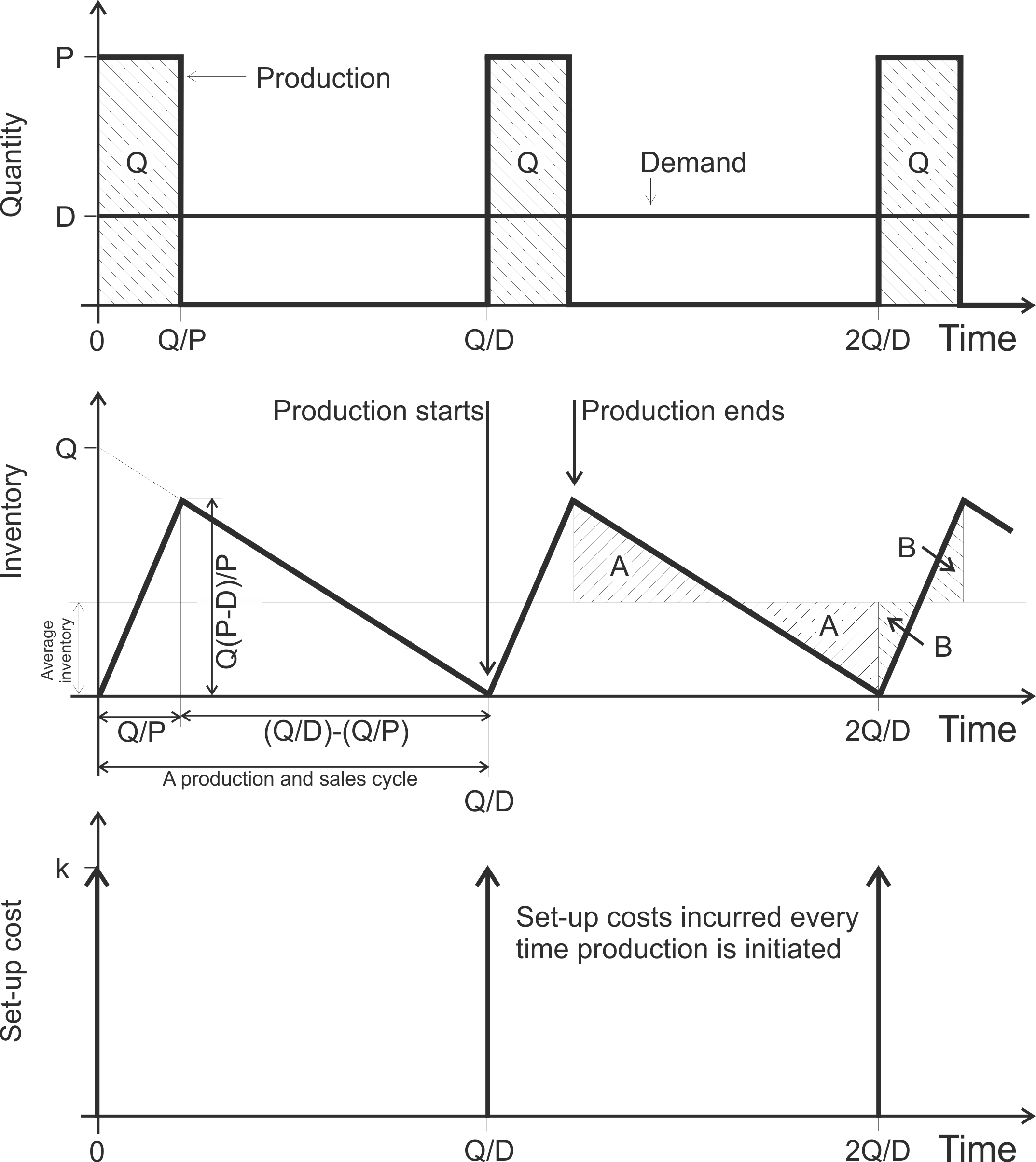

Figure 4.16: Production, inventory, and set-ups over time in the EPQ model

Adding together the three cost components, we obtain the following expression for the total annual costs, \[\begin{align} TC=\frac{Dk}{Q}+\frac{Qh(P-D)}{2P}+cD. \end{align}\] Taking the derivative of \(TC\) with respect to \(Q\) yields \[\begin{align} \frac{dTC}{Q}=-\frac{Dk}{Q^2}+\frac{h(P-D)}{2P}. \end{align}\] Setting the derivative to zero and solving for the optimal batch quantity, gives \[\begin{align} \tag{4.29} Q^\star=\sqrt{\frac{2PDk}{h(P-D)}}=\sqrt{\frac{2Dk}{h}}\sqrt{\frac{P}{P-D}}. \end{align}\] We can verify that \(Q^\star\) in (4.29) is a minimum by taking the second derivative, \(\frac{d^2TC}{dQ^2}=-\frac{2Dk}{q^3}\). As the second derivative is always positive (due to \(\{Q,D,k\}>0\)), \(Q^\star\) is a minimum.

Table 4.9 provides a summary of properties of the EPQ model.

Table 4.9: Properties of the EPQ model

EPQ property	Formula
The economic production quantity	\(Q^\star = \sqrt{\frac{2 P D k}{h(P-D)}}\)
Number of set-up per year	\(D/Q\)
Time between set-ups (assuming 365 working days per year)	\(365 \times Q/D\)
Total annual costs	\(\frac{Qh(P-D)}{2P}+Dk/Q+cD\)
Annual inventory holding cost	\(\frac{Qh(P-D)}{2P}\)
Annual set-up cost	\(Dk/Q\)
Annual production cost	\(cD\)
Minimum inventory held	0
Maximum inventory held	\(Q(P-D)/P\)
Average inventory held	\(\frac{Q(P-D)}{2P}\)

Example calculation of the EPQ and characteristics of the solution Let us assume the following set of costs and annual demand and production rates exist:

• Annual cost of holding one unit of inventory, \(h=73\).
• Cost of placing an order, \(k=10\).
• Unit production cost, \(c=1\).
• Annual demand, what is sold in a complete year (365 days), \(D=1460\).
• Annual production rate, what would be produced if the production system ran continuously for a complete year (365 days), \(P=2920\).

Using the formula in Table 4.9,the following information can be gathered about the EPQ problem:

• Economic production quantity, \(Q^\star = \sqrt{\frac{2 P D k}{h(P-D)}}=\sqrt{\frac{2\times 2920 \times 1460\times 10}{73(2920-1460)}}= 28.28\).
• Number of set-ups per year = \(D/Q=1460/28.28=51.62\).
• Time between set-ups = \(365 \times Q/D = 365 \times 28.28/1460=12.9\) days.
• Annual inventory holding costs = \(\frac{Qh(P-D)}{2P}=\frac{28.28\times 73(2920-1460)}{2(2920)}=£516.19\).
• Annual set-up costs = \(Dk/Q=1460(10)/28.28=£516.19\).
• Annual production costs =\(cD=1(1460)=£1460\).
• Annual costs = \(\frac{Qh(P-D)}{2P}+Dk/Q+cD=\frac{28.28 \times 73(2920-1460)}{2(2920)}+1460(10)/28.28+1(1460)=£2492.38\).
• Minimum inventory = 0 (from the assumptions made about the EPQ model).
• Maximum inventory = \(Q(P-D)/P=28.28(2920-1460)/2920=14.14\).
• Average inventory = \(\frac{Q(P-D)}{2P}=\frac{28.28(2920-1460)}{2(2920)}=7.07\).

A Shiny App is available here where we can explore the EPQ model interactively. The App can calculate \(Q^\star\) automatically, plot the total cost graph, as well as deal with any rounding and batching issues.

4.5.2 Managerial insights from the EPQ model

Reducing the set-up cost \(k\) results in smaller production quantities \(Q_{EPQ}^\star\). Furthermore, increasing the production rate \(P\) results in smaller \(Q_{EPQ}^\star\). The order quantity in the EPQ decision is always larger than the order quantity under the EOQ decision¹⁷, that is, \(Q^\star_{EPQ}> Q^\star_{EOQ}\) as \(\sqrt{P/(P-D)}>1\) when \(P>D\). In order for the production system to be able to keep up with demand the production rate must be larger than the demand rate, \(P>D\). Furthermore, as the annual demand \(D\) approaches \(P\) (from below) then \(Q^\star_{EPQ}\) gets larger. When \(D = P\), \(Q^\star_{EPQ}\rightarrow \infty\) indicating that production is continuous and never ceases. As \(P\rightarrow \infty\), indicating that complete orders arrive instantaneously, then \(Q^\star_{EPQ}=Q^\star_{EOQ}\). That is, the EPQ model degenerates into the EOQ model, see Chapter 6. When the net present value (NPV) of the cash flows resulting from the replenishment decision are considered, \(Q^\star_{EPQ}\) gets smaller as the interest rate in the NPV calculation gets larger, Disney, Warburton, and Zhong (2013).

Finally, let’s consider some practical issues with EPQ decisions. Over time, the engineering department may have made changes to the way a changeover is completed (perhaps some kaizen activities have made the changeover quicker/cheaper), the demand or production rates may have changed, or the material, labour and storage costs may have changed. Periodically, in order to gain the full benefit from these hard earned improvements, we should revisit the assumed data behind the EPQ decision and update the order quantity.

Having now calculated the system recommended production targets, the next chapter considers how to: gain approval for the production planning from important internal stakeholders via a weekly production planning meeting, communicate that plan to the shop floor, and how to ensure what was agreed upon is actual produced.

References

Boute, R., S. M. Disney, J. Gijsbrechts, and J. A. Van Mieghem. 2022. “Dual Sourcing and Smoothing Under Non-Stationary Demand Time Series: Re-Shoring with SpeedFactories.” Management Science 68: 1039–57. https://doi.org/10.1287/mnsc.2020.3951.

Dejonckheere, J., S. M. Disney, M. R. Lambrecht, and D. R. Towill. 2003. “Measuring and Avoiding the Bullwhip Effect: A Control Theoretic Approach.” European Journal of Operational Research 147 (3): 567–90. https://doi.org/10.1016/S0377-2217(02)00369-7.

Disney, S. M., A. Maltz, X. Wang, and R. D. H. Warburton. 2016. “Inventory Management for Stochastic Lead Times with Order Crossovers.” European Journal of Operational Research 248 (2): 473–86. https://doi.org/10.1016/j.ejor.2015.07.047.

Disney, S. M., R. D. H. Warburton, and Q. C. Zhong. 2013. “Net Present Value Analysis of the Economic Production Quantity.” IMA Journal of Management Mathematics 24 (4): 423–35. https://doi.org/10.1093/imaman/dpt002.

Harris, F. W. 1913. “How Many Parts to Make at Once.” Factory, The Magazine of Management 10: 135–36, 152. http://www.jstor.org/stable/170961.

Li, Q., S. M. Disney, and G. Gaalman. 2014. “Avoiding the Bullwhip Effect Using Damped Trend Forecasting and the Order-up-to Replenishment Policy.” International Journal of Production Economics 149: 3–16. https://doi.org/10.1016/j.ijpe.2013.11.010.

Li, Q., G. Gaalman, and S. M. Disney. 2023. “On the Equivalence of the Proportional and Damped Trend Order-up-to Policies: An Eigenvalue Analysis.” International Journal of Production Economics 265: 109005. https://doi.org/10.1016/j.ijpe.2023.109005.

Michna, Z., S. M. Disney, and P. Nielsen. 2019. “The Impact of Stochastic Lead Times on the Bullwhip Effect Under Correlated Demand and Moving Average Forecasts.” Omega 93: 102033. https://doi.org/10.1016/j.omega.2019.02.002.

Wang, X., S. M. Disney, and J. Wang. 2012. “Stability Analysis of Constrained Inventory Systems with Transportation Delay.” European Journal of Operational Research 223 (1): 86–95. https://doi.org/10.1016/j.ejor.2012.06.014.

---

14. The initial condition for the inventory is randomly chosen to be 8 in this example.↩︎

15. Periods -1 and 0 have been omitted from the variance calculations as they represent initial conditions. These variance were obtained using the “=VARP()” function in Excel. That is, they assume the data in periods 1 to 10 represent the whole population.↩︎

16. The EOQ formula is one of the first theories for managing inventory, dating back to Ford W. Harris (1913). There have been possibly hundreds of extensions, refinements and elaborations to the original model, but we will consider only the original EOQ formula and the EPQ formula herein.↩︎

17. The EOQ model is used when the whole order arrives at the same instant, perhaps when product is deliver by a supplier into our raw material inventory. For this reason, we review the EOQ model in Chapter 6.1.↩︎