Chapter 6 Giving your suppliers orders and future guidance

Figure 6.1: This chapter is currently under construction, it will probably be ready in week 8 or 9 of the semester. Please come back later
Map of the chapter is required here
The final stage of the planning cycle is to issue call-off and forecast orders to your suppliers. The call-off orders are instructions to your supplier about what to deliver in the current period. The forecast orders are guidance, a prediction but not a guarantee, of the requirements in the future. The call-off and order forecasts can be issued by your ERP system, although some companies do this via fax, EDI or email.
The forecast orders for the MRP module can come from either the Planning module or the Scheduling module. The purchasing department maintains lead-time information in the MRP module. Q. How do they know it is correct? It is important, to get at least the average lead-time right, even if you have a stochastic lead-time. Often companies presume that erring on the side of caution and high-balling the lead-time is the best option but this result in excess inventory. Perhaps the logistics department should be informing the purchasing department what the actual lead-times are (monitor them and report deviances.) these are ideas that need to be addressed
Some suppliers may be under a VMI contract to supply your factory. Here no safety stock is maintained in the MRP system, but current inventory levels and order forecasts may be passed to the supplier so that they may infer recent usage from the net change in inventory levels as well as giving them guidance for long-term capacity planning. VMI suppliers may be delivering to an open purchase order with a large quantity and no financial information. Otherwise, the receiving dock may turn away the undocumented supply. Suppliers on a regular supply chain contract by given firm call-off orders and a purchase-order each period and guidance on future orders. Items brought from a spot market may still require an MRP process to exist, if only for your long term financial planning activities.
6.1 Economic order quantity
A useful tool to deter how much to order from suppliers is the economic order quantity (EOQ) model. The EOQ model determines how much to order so as to minimize some (defined, assumed) costs. The costs involved are usually order placement costs and inventory holding costs. Order placement costs are the cost of placing an order plus the cost to deliver and receive that order (so transportation and unloading costs are included here). The basic idea is that we want to minimize the sum of the order placement and inventory holding costs. In order to minimize order placement costs, we place large orders so that there is a long time between placing orders and we order less frequently. In this case, we would incur less order placement costs. However, placing large orders means that we have, on the average, more inventory in our warehouse (or on the shelf/in the shop). This inventory is expensive, and there is an opportunity cost involved in financing the inventory. So there is a trade-off to be made. We could place small orders and have low inventory costs, but high order placement costs. Alternatively, we could place large orders resulting in high inventory costs, but the order placement costs have been reduced. The EOQ decision minimizes the sum of these two costs.
The EOQ formula. The economic order quantity is given by
\[\begin{align} Q^\star=\sqrt{\frac{2 D k}{h}} \end{align}\]
where
- \(Q\) = the order quantity. The optimal \(Q\), the order quantity that minimizes the total cost, is \(Q^\star\).
- \(k\) = cost of placing an order. Sometimes this is called the set-up cost. We assume that this is independent of the order quantity and does not change over the year.
- \(h\) = cost of holding one unit of inventory for one year, assumed to be a constant.
- \(D\) = annual demand. This is what is sold in a complete year (365 days). We assume that the demand rate is spread out evenly throughout the whole year.
The EOQ model is a mathematical model that relies on some assumptions. These assumptions are:
- Annual demand is known, or is forecast-able.
- The daily demand is constant, distributed evenly over each day of the year.
- Orders are received complete, all at once, after a known and constant lead-time.
- Stock-outs (or backlogs) are avoided by ordering on time.
- There are no quantity discounts (although this can be easily handled using standard techniques – see a good operations management textbook).
- The only costs are the ordering (or set-up) and the inventory holding (storage) costs.
- All costs are known and constant.
- The set-up cost is independent of the order quantity.
- Only a single product is considered.
We have assumed the demand rate is known and constant then the inventory will fall over time at a constant rate equal to the demand rate, see Figure 6.2. When the inventory level falls to the re-order point \(R\), a new order is placed (for a cost of \(k\)) to replenish the inventory. This order is for \(Q\) products that will arrive \(L\) time-periods after the order was placed. As \(L\) is assumed to be known and constant, and as demand is known and constant, then the order will arrive and replenish inventory at the moment the inventory level reaches zero. The receipt of the order brings the inventory level back up to \(Q\), from which the replenishment cycle continues. Each replenishment cycle lasts \(Q/D\) years, the number of orders placed in a year is \(D/Q\).
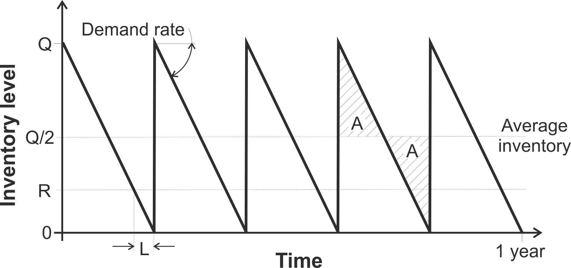
Figure 6.2: The inventory behavior over time in the EOQ model
Deriving the optimal order quantity in an EOQ decision
The annual order cost is \(Dk/Q\), which is decreasing in \(Q\). The average inventory of \(Q/2\) can easily be seen in Figure 6.2 by noting that the two areas labelled ‘A’ are equal. The annual inventory holding cost is \(Qh/2\), which is linearly increasing in \(Q\). Adding these two costs together gives a total annual cost, \(TC\), of \[\begin{align} TC=\frac{Qh}{2}+\frac{Dk}{Q}. \end{align}\] As the inventory cost is increasing in \(Q\) and the order cost is decreasing, there is a minimum \(TC\) for a particular optimal \(Q^\star\). We can find the \(Q^\star\) that minimizes \(TC\) from the first order conditions. Differentiating \(TC\), with respect to \(Q\) provides the gradient, \[\begin{align} \frac{dTC}{Q}=\frac{h}{2}-\frac{Dk}{Q^2}. \end{align}\] The optimal \(Q^\star\) can be found by setting the gradient to zero, \[\begin{align} \frac{h}{2}-\frac{Dk}{Q^2}=&0, \end{align}\] adding \({Dk}/{Q^2}\) to both sides, \[\begin{align} \frac{Dk}{Q^2}=&\frac{h}{2}, \end{align}\] cross-multiplying the denominators, \[\begin{align} 2Dk=& Q^2 h, \end{align}\] and finally dividing both sides by \(h\) and taking the square root, \[\begin{align} Q^\star=& \sqrt{\frac{2Dk}{h}}. \end{align}\] At this stage we have no knowledge of whether \(Q^\star\) is a maximum, a minimum, or an inflection point. We can resolve this ambiguity by inspecting the second derivative of the total cost expression. The second derivative is, \[\begin{align} \frac{d^2TC}{dQ^2}=\frac{2Dk}{Q^3}. \end{align}\] As \(\{D,k,h\}>0\) then the second derivative is always positive which implies that \(Q^\star\) is a minimum. Table 6.1 provides a summary of properties of the economic order quantity model.
| EOQ property | Formula |
|---|---|
| The economic order quantity | \(Q^\star = \sqrt{2 D k/h}\) |
| Number of orders placed each year | \(D/Q\) |
| Days between placing orders (assuming 365 working days per year) | \(365 \times (Q/D)\) |
| Total annual costs | \((Dk/Q)+(Qh/2)\) |
| Annual inventory holding cost | \(Qh/2\) |
| Annual ordering cost | \(Dk/Q\) |
| Minimum, maximum and average inventory held | Min = 0, Max = \(Q^\star\), Average = \(Q^\star /2\) |
| Total cost per replenishment cycle | \(2k\) |
6.1.1 Managerial insights from the EOQ model
Figure 6.3 provides a sketch of the costs in the EOQ model as a function of the order quantity \(Q\). We can see that the annual inventory holding costs are a linear function of \(Q\) and the annual order placement costs are a convex decreasing function of \(Q\). The total costs, the sum of the inventory and order placement costs, is a convex function have a minimum, or optimum, \(Q\). The total cost curve only increases slowly near \(Q^\star\), indicating that the small deviations from the optimal quantity will not significantly increase costs; that is, the EOQ model is quite robust. Also, if a different \(Q\) to \(Q^\star\) are required, then it may be better to use slightly larger \(Q\), rather than slightly smaller \(Q\). However, if rounding \(Q^\star\) to an integer (or box, crate, or bag size) then we should calculate the costs for rounding up, and for rounding down, as it is often not possible to determine which direction to move beforehand.
 A Shiny App is available here where we can explore the EOQ model interactively. The App can calculate \(Q^\star\) automatically, plot the total cost graph, as well as deal with any rounding and batching issues.
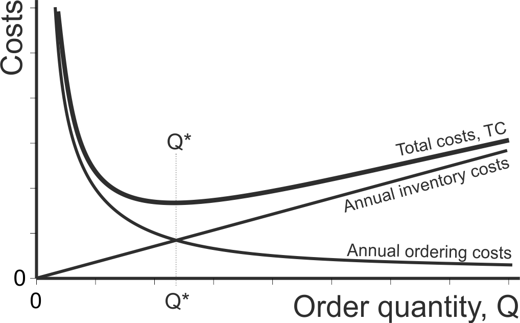
Figure 6.3: The components of the total cost in an EOQ problem
Increasing the order quantity increases the average cycle stock. In fact, the average inventory is \(Q/2\). Large batch sizes are also an important cause of the bullwhip problem. However, there is a trade-off between the ordering-up cost and holding cost. The holding cost is largely determined by the value of the inventory and the cost of capital. Both of these factors are rather uncontrollable (and if they were controllable higher inventory costs and cost of capital would be required to reduce batch sizes, not a readily accepted course of action). However, reducing the ordering-up costs (\(k\)) results in smaller batch sizes and lower inventories, hence the importance of the Single Minute Exchange of Dies (SMED) concept, see Chapter 5. Note, that there is a square root relationship between \(Q\) and \(k\). This means that if the ordering-up cost reduces by a factor of 4 the batch size decreases by a factor of 2.
There is also a square root relationship between \(Q\) and \(D\). Four-fold increases in demand result in batch sizes that are twice as large and are produced twice as often. This means that inventory should not track sales growth and brings into doubt the usefulness of the Days of Sales and the Inventory Turnover metrics. For example, 100% growth in sales can be sustained by a mere 41% (from the square root of 2) increase in cycle inventory. This relationship between \(Q\) and \(D\) also has an influence on centralization decisions and component commonality due to economies of scale.
The EOQ is likely to introduce order variability into the system. Bullwhip ratios can be reduced when the batch sizes are a factor (or multiple) of the average demand, see Potter and Disney (2006). For example, if the average demand was 100, producing in quantities of 1, 2, 4, 5, 10, 20, 25, 50, 100, 200, 300, 400,… will minimize the resulting Bullwhip. The Bullwhip measure will be particularly large at the mid-points between these values (1.5, 3, 4.5, 7.5, 15, 22.5, 37.5, 75, 150, 250, 350,… for example).
It is also interesting to note that if one considers the time value of money in a net present value analysis, then the optimal \(Q\) maintained by both the EOQ (and the EPQ approaches, see Section 4.5) becomes smaller, see Disney and Warburton (2012) and Disney, Warburton, and Zhong (2013). Thus, in environments where the cost of capital or inflation is high, then reducing the batch quantity \(Q\) is a good option. In other situations, the batch size is not driven by a cost minimization procedure, but other factors such as case/crate/bag sizes, or the number of items that a machine produces in one cycle. Alternatively, a minimum order quantity could be imposed, or quantity discount offered, by a supplier.
6.1.2 When to place an order: The re-order point
Having decided on the quantity to order from your supplier, the next question is when to place your order. We release the order to the supplier, when the inventory level fall to a pre-determined level called the re-order point.
Under a constant demand and lead-time, the re-order point \(R=\lceil \mu_{d}L \rceil\), where \(\mu_{d}\) is average the daily demand, \(L\) is the replenishment lead-time in days and \(\lceil \cdot \rceil\) is the ceiling operator (that is, around any fractional number up to the next integer). If the demand over the replenishment lead-time was normally distributed (the central limit theorem suggests that the lead-time demand distribution will become more like the normal distribution as the lead-time increases) then the re-order point will be given by \[\begin{align} R=\lceil \mu_{d}L+z \sigma_L \rceil \end{align}\] where \(z\) is a safety factor linked to your target availability and \(\sigma_l\) is the standard deviation of the lead-time demand. The safety factor, \(z = \Phi^{-1}[x]\), is the inverse of the cumulative density function of the standard normal distribution evaluated at \(x\), the proportion of inventory cycles that end without incurring a stock-out.
A Shiny App is available here where we can explore the standard normal distribution interactively. The App can calculate the PDF, the CDF and the Loss function and their inverses for the standard normal distribution.
For example, suppose that we wished 90% of inventory cycles do not experience a stock-out then we enter 0.9 into the query box for the inverse of the cumulative density function (CDF) on the left hand panel and look for the answer under the CDF graph in the main panel; \(z = 1.28155\).
Example calculation of the re-order point.
Suppose that daily demand is as given in the second column of Table 6.2, 95% of inventory cycles should end with positive inventory, and the lead time, \(L=5\). To calculate the re-order point, we first we average the daily demand to find \(\mu_{d}\). Next, we aggregate the daily demand into lead time demand. This is done by simply summing the last five observed demand points, see the third column of Table 6.2. The average lead-time demand is then found to be \(\mu_{l}=25\). Using \(\mu_{d}\) we can then determine the per period contribution to the variance calculation in the fourth column, which we average to obtain the variance of the lead-time demand, \(\sigma^2_l=17\).
| Time, \(t\) | Demand, \(d_t\) | Demand over the lead time, \(\sum_{i=0}^4 d_{t-i}\) | Variance calculation, \((\mu_L-d_t)^2\) |
|---|---|---|---|
| 1 | 3 | - | - |
| 2 | 0 | - | - |
| 3 | 6 | - | - |
| 4 | 6 | - | - |
| 5 | 5 | \(3+0+6+6+5=20\) | \((25-20)^2=25\) |
| 6 | 9 | \(0+6+6+5+9=29\) | \((25-26)^2=1\) |
| 7 | 6 | \(6+6+5+9+6=32\) | \((25-32)^2=49\) |
| 8 | 3 | \(6+5+9+6+3=29\) | \((25-29)^2=16\) |
| 9 | 7 | \(5+9+6+3+7=30\) | \((25-30)^2=25\) |
| 10 | 0 | \(9+6+3+7+0=25\) | \((25-25)^2=0\) |
| 11 | 6 | \(6+3+7+0+6=22\) | \((25-22)^2=9\) |
| 12 | 3 | \(3+7+0+6+3=19\) | \((25-19)^2=36\) |
| 13 | 6 | \(7+0+6+3+6=22\) | \((25-22)^2=9\) |
| 14 | 10 | \(0+6+3+6+10=25\) | \((25-25)^2=0\) |
| Average | \(\mu_d=5\) | \(\mu_L=25\) | \(\sigma^2_L=17\) |
For 95% availability a z-factor of \(z = 1.64485\) is required. Finally, we have all of the components to the re-order point calculation; \[\begin{align} R=\lceil\mu_{d}L+z \sigma_L \rceil= \lceil 25+1.64485\sqrt{17}\rceil=\lceil 131.78 \rceil = 132. \end{align}\]
The EOQ/re-order point mechanism requires some sort of inventory level monitoring system to be in place. Your ERP system by have this function built into a detailed scheduling module. If you are not using an ERP system to control this, then you will need to set up some sort of manual process to monitor the inventory levels and to trigger the replenishment decision. This could be done using some sort of two-bin or Kanban system.
6.1.3 EOQ with volume discounts
Often suppliers will offer volume-based price discounts in order to encourage customers to place larger orders. This calls for an important extension to the EOQ model. Presumably the purchase price is reduced if more products are ordered. See Figure 6.4, where a different price per item is charged depending on the quantity ordered. Here the price \(p_0\) is charged if the order size is between \(0<Q<Q_1\) and \(p_i\) if \(Q_i\leq Q<Q_{i+1}\). Presumably \(p_i\) is decreasing in \(i\), that is \(p_0<p_1<p_2<\dots\).
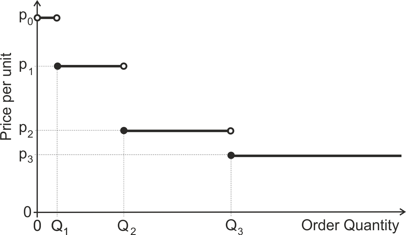
Figure 6.4: Price discounts for different ordering quantities
The procedure to determine the EOQ in situations with volume discounts is outlined below.
Procedure for determining the EOQ with volume discounts
Step 1. For each discount level calculate \[\begin{align} \tag{6.1} Q^\star=\sqrt{\frac{2Dk}{ip}}, \end{align}\] the EOQ formula for volume discounts.
Step 2. If \(Q^\star\) is too low for a particular discount then adjust \(Q^\star\) upward to the lowest quantity that will qualify for the discount. \(Q^\star\)’s that are too high may be discarded.
Step 3. Compute the total cost for every remaining \(Q^\star\) (remembering it may have be adjusted).
Step 4. Select the (adjusted) \(Q^\star\) that has the lowest total cost.Notice, that the EOQ formula with volume discounts is slightly different to the usual EOQ formula. Specifically, the unit holding cost is now proportional to the purchase price, \(p\). That is, we assume the per unit annual holding cost, \(h=ip\), is a proportion \(i\) of the purchase price \(p\). This allows the per unit inventory holding cost to change with purchase price, which depends on the volume purchased. \(i\) is a proportion of the purchase price used to determine the holding cost. \(i\) could be linked to the cost of capital that your company incurs when it borrows money to fund its business. The proportion \(i\) is also often inflated so that costs of warehousing, insurance, damage, shrinkage, for example are based on their value (purchase price). Thus, it is often the case that \(i\) is as high as 0.2 to 0.3.
Equation (6.1) is used to generate several \(Q^\star\), one for each volume discount, which are the minimum of the total cost curves for the different purchase costs \(p_i\) in Figure 6.5. Some of these \(Q^\star\) may be valid; that is they lie within the relevant volume range to obtain that price. Other \(Q^\star\)s may be invalid in the sense that ordering the prescribed quantity does not allow the items to be purchased at the price used in the EOQ equation (6.1), see Figure 6.5.

Figure 6.5: Total costs when quantity discounts exist
If a \(Q^\star\) is below the volume required to access price \(p_i\) then \(Q^\star\) is adjusted upward to the lowest quantity that will qualify for the discount, and you proceed to calculate the total cost (that should now include the purchase cost of the items). \(Q^\star\)s that are above the volume range to access a particular price may be discarded. This is because if you actually order that amount, you will actually be offered an even lower purchase price, so \(Q^\star\)s below the volume range will never be optimal.
Let’s illustrate how this procedure works by example.
Example: The economic order quantity with volume discounts at Quick Repair Garages
Let’s consider the fictional case of Quick Repair Garages who replace car tyres. One particular tyre has an annual demand of \(D=1000\) units. It costs Quick Repair Garages \(k=£40\) to place the order for tyres and have them delivered by the supplier, regardless of the number of tyres ordered. Quick Repair Garages fund their business with a commercial loan with an interest of 20% per year (\(i=0.2\)). The supplier, in order to increase sales, offers a volume-based price discount depending on the quantity of tyres in each order. The percentage price discount from the nominal price for a single tyre of \(p_0=£10\) is given in Table 6.3.
| Quantity ordered | Discount |
|---|---|
| 1 to 99 | 0% |
| 100 to 199 | 2.5% |
| 200 to 299 | 5% |
| 300+ | 6% |
How may tyres should Quick Repair Garages order in each delivery? What is the total annual cost with this order quantity? How many orders are placed per year?
Solution procedure
Step 1. For each discount level calculate \(Q^\star\) using the EOQ formula for volume discounts.
First, reading the question we see that the annual demand \(D=10\) and the cost of placing an order is \(k=£40\). The cost of capital is 20%, so \(i=0.2\). The nominal cost of a tyre is \(p_0=£10.00\). Thus, if we order 1 to 99 tyres then the price per tyre would be \(p_0=£10.00\). Ordering between 100 and 199 also us to obtain a 2.5% discount, so the cost per tyre would be \(p_1=£9.75\). The cost per tyre for order quantities between 200 and 299 is \(p_2=£9.50\) and for 300 and above the unit purchase is \(p_3=£9.40\).
Next we use (6.1) to calculate the \(Q^\star\) for each of the volume / price discount ranges. For the 1-99 range the calculation is \(Q^\star=\sqrt{\frac{2 \times 1000 \times 40}{0.2 \times 10}}=200\). We notice that the only number that changes with each calculation is the unit purchase price, \(p_i\).
| Quantity ordered | Discount | Purchase price, \(p\) | \(Q^\star\) |
|---|---|---|---|
| 1-99 | 0% | £10.00 | \(Q^\star=\sqrt{\frac{2 \times 1000 \times 40}{0.2 \times 10}}=200\) |
| 100-199 | 2.5% | £9.75 | \(Q^\star=\sqrt{\frac{2 \times 1000 \times 40}{0.2 \times 9.75}}=202.55\) |
| 200-299 | 5% | £9.50 | \(Q^\star=\sqrt{\frac{2 \times 1000 \times 40}{0.2 \times 9.5}}=205.20\) |
| 300+ | 6% | £9.40 | \(Q^\star=\sqrt{\frac{2 \times 1000 \times 40}{0.2 \times 9.4}}=206.28\) |
Step 2. Adjust the \(Q^\star\)s if needed to fit into volume range or if integer/batch quantities are needed
We notice that three of the \(Q^\star\) calculated in step 1 fall outside of the volume range that the discount is applied to. If \(Q^\star\) is too low for a particular discount then we must adjust \(Q^\star\) upwards to the lowest quantity that will qualify for the discount. \(Q^\star\)s that are too high may be discarded.
| Quantity ordered | Discount | Purchase price, \(p\) | \(Q^\star\) | Adjusted \(Q^\star\) |
|---|---|---|---|---|
| 1-99 | 0% | £10.00 | \(200\) | Discard |
| 100-199 | 2.5% | £9.75 | \(202.55\) | Discard |
| 200-299 | 5% | £9.50 | \(205.20\) | 20519 |
| 300+ | 6% | £9.40 | \(206.28\) | 300 |
Step 3. Compute the costs for every remaining \(Q^\star\).
Using the adjusted \(Q^\star\), for each of the volume discounts that has not been discarded, we calculate the ordering cost, the inventory carrying cost and the purchase cost. The annual ordering cost is given by
\[\begin{align} \tag{6.2} \text{Ordering cost}=\frac{Dk}{Q} \end{align}\]
as before in the traditional EOQ approach. The annual inventory cost is given by
\[\begin{align} \tag{6.3} \text{Inventory cost}=\frac{Qip}{2} \end{align}\]
which is slightly different as the holding cost is expressed as proportion \(i\) of the purchase cost, \(p\). As the purchase price is also changing due to the quantity ordered we also have to calculate the annual purchase cost,
\[\begin{align} \tag{6.4} \text{Purchasing cost}=pD \end{align}\]
Using (6.2), (6.3) and (6.4) we calculate the ordering, carrying and purchase cost as follows. We also sum these three costs to give a Total Annual Cost for each of the discount bands as shown in the last column of Table 6.6.
| Quantity ordered | Purchase price, \(p\) | Adjusted \(Q^\star\) | Ordering cost, \(\frac{Dk}{Q}\) | Inventory cost, \(\frac{Qip}{2}\) | Purchase cost, \(pD\) | Total annual cost |
|---|---|---|---|---|---|---|
| 1-99 | £10.00 | Discard | - | - | - | - |
| 100-199 | £9.75 | Discard | - | - | - | - |
| 200-299 | £9.50 | 205 | £195.12 | £194.75 | £9500.00 | £9889.87 |
| 300+ | £9.40 | 300 | £133.33 | £282.00 | £9400.00 | £9815.33 |
Step 4. Finally we select the adjusted the \(Q^\star\) that has the lowest Total Annual Cost. That is, we select \(Q^\star=300\). The minimised Total Annual Cost is £9815.33 and there \(\frac{D}{Q^\star}=\frac{1000}{300}=3.33\) orders placed each year.
6.2 Material requirements planning
Dependent demand, independent demand
6.2.1 Bill of materials
BOM is also known as a Production Process Module, Product Data Structure.
Figure 38. An example BOM (Perhaps an IKEA product?)
The BOM information in your MRP system needs to be correct. Over time, engineering changes will be made to the product as components are modified and recipes improved. This whole engineering change process requires careful management. Quality losses, scrap, and yield rates need to be monitored and your MRP system updated with the latest information. Lead-times may change when parts are sourced from different vendors. Suppliers may move the location of their production activities or use different transportation lanes.
It is critical to use the correct units of measurements in the MRP system. For example, some countries still use pounds and ounces for weight instead of kilograms or feet and inches instead of meters and centimetres. A British ton (or long ton) is 1016.047kg, the U.S. ton (or short ton) is 907.1847kg, and a metric ton (or tonne) is a 1000kg. The imperial gallon is 4546cc. The U.S. liquid gallon is 3785.41cc or approximately 3.785cc. The U.S. dry gallon is 4405cc. These small differences in definition can really mess up a supply chain and mistakes do occur.
6.2.2 MRP nervousness
Explain what MRP nervousness problem in here.
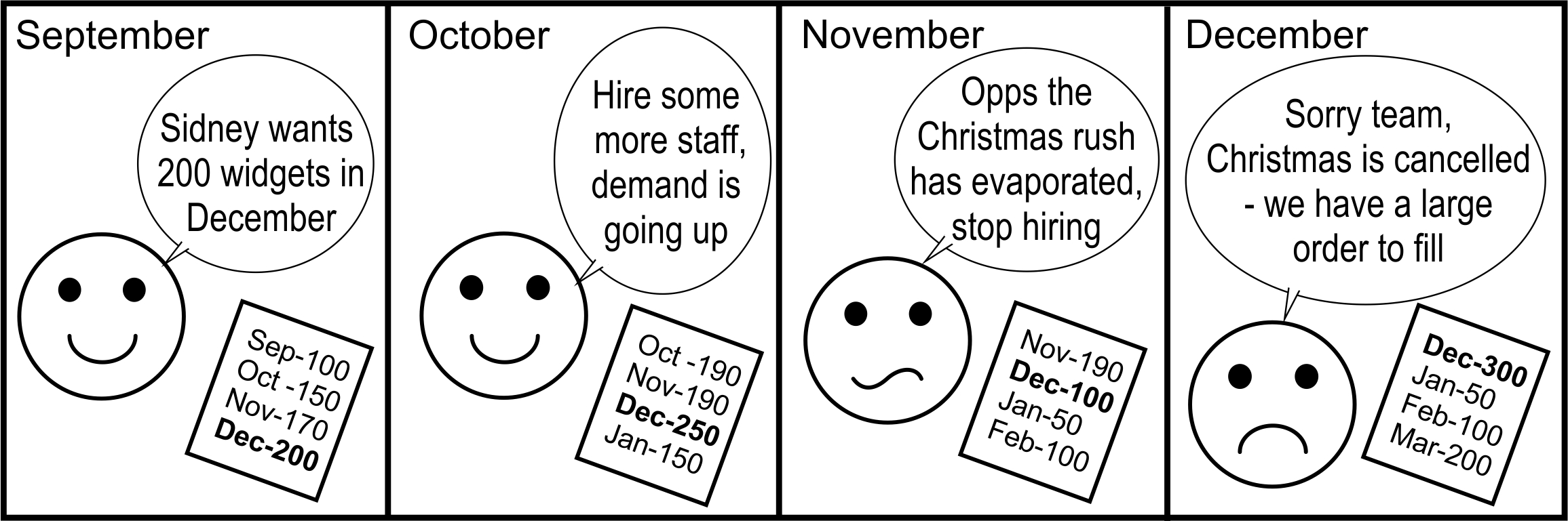
Figure 6.6: MRP nervousness: Rescheduling the schedules you just rescheduled
Quantity Demand forecast for delivery in week
Table 33. Example MRP data (Call-off orders in bold)
| First Header | Second Header | Third Header |
|---|---|---|
| Content | Long Cell | |
| Content | Cell | Cell |
| New section | More | Data |
| And more | With an escaped ‘|’ |
The demand experienced by the supplier each week (the call-off orders) is highlighted in bold in Table 33. The variance of the supplier’s demand is part of the bullwhip calculation, and we find them as the bold numbers lying on the diagonal in Table 33. The supplier’s demand was 120 in week 0, 80 in the week -1 , 90 in the week -2, 110 in the week -4 and 100 in the week -5 and so on. Demand fluctuates from week to week. We can also see another form of uncertainty in Table 33. The forecasts of the call-off orders made in previous weeks were both inaccurate and are also variable from week to week. For example, in week -1, the forecast of the supplier’s demand in week 0 was 101. However, when week 0 comes along, the actual call-off order was only 120. The forecast of the demand in the week -1, made in the week -2, was 122; the forecast made in the week -2 was 103. This type of forecast uncertainty is an effect known as MRP nervousness. The numbers here need to be carefully checked.
Table 34. Example calculation of the MRP nervousness measure with Exponential Smoothing forecasts
Suppliers would like to have accurate predictions of future demand so that they may set-up their supply chain to meet future demand. This may mean ordering raw materials, hiring staff, installing production capacity (machines, etc.) as well as producing the quantity required. If the forecast is too high, then perhaps the supplier has ordered too much raw material, made too much product, or hired too many staff, etc. If the forecasts are too low, perhaps the supplier did not order enough raw material or must work overtime with the smaller than required workforce he has in place. We can see then that it is just not the variability of the amount of work that has to be done; the predictability of the work required is also important.
To manage this MRP nervousness effect, we need a measure of the nervousness. We do this by first calculating the variance of the j-step ahead order forecast error with
\[\begin{align} \Delta[j]=\lim_{T\to\infty}\left( \frac{1}{T}\sum_{i=0}^T \left( \hat{O}_{t-j-i,t-i}-O_{t-i} \right)^2 \right) \end{align}\]
Imagine it is now time \(t=0\) in Table 33 with \(j=1\), the one period ahead order forecast error is given by
\[\begin{equation} \Delta[1]=\frac{1}{5}\left((82-120)^2+(122-80)^2+(120-90)^2+(112-110)^2+(102-100)^2\right)=672 \end{equation}\]
As a forecast error in the near future is likely to be more costly than one in the distant future, and as a large forecast error is more expensive than a small error, an exponentially weighted sum of order forecast error variances is a natural measure of nervousness:
Here the exponential weighting factor, \(w\), determines how quickly the variability of the future order forecast errors decay away (in much the same way as the forecasting parameter in exponential smoothing behaves). When \(w\) is large, the influence of the forecast error decays away more quickly than when \(w\) is small. When \(0<w<1\), the sum in (22) converges to a finite number, allowing us to measure the nervousness produced by different replenishment system designs. Lower \(\Delta\) indicate more accurate future guidance (that is, less nervousness is created), and the easier it will be for your suppliers to organize their activities to meet demand.
| j | \(\Delta[j]\) | \(w(1-w)^{j-1}\) | \(w(1-w)^{j-1}\Delta[j]\) |
|---|---|---|---|
| 1 | 561 | 0.5 | 280.5 |
| 2 | 672 | 0.25 | 168 |
| 3 | 689 | 0.125 | 86.125 |
| 4 | 696 | 0.0625 | 43.5 |
| 5 | 705 | 0.03125 | 22.03125 |
| 7 | 748 | 0.015625 | 11.6875 |
| Total | \(\Delta=611.84\) |
What about bias and gaming? Bias in the order forecasts is also important. If the future guidance is based on the planning book forecasts, and the manual interventions in the forecasts are minimal the bias in the MRP order forecast should be minimal. People have a tenancy to communicate an inflated forecast to a) secure supply by tricking the supplier to invest in extra capacity, b) improve their position in pricing negotiations.
OUT policy uses the forecasts from the forecasting system POUT policy can use the PFG mechanism
\[\begin{equation} \hat{o}_{t,t+j}=\hat{d}_{t,t+T_s+1+j}+\frac{1}{T_i}\left(\frac{T_i-1}{T_i}\right)^j \left( TNS-ns_t+\sum_{i=1}^{T_s}\left(\hat{d}_{t,t+1}-o_{t-1}\right)\right) \end{equation}\]
Month versus weeks, long versus short Capacity limited
The cost of the MRP nervousness
- Add some typical costs in here
- and some more costs
- Demands greater then the forecasts within the lead-time result in lower inventory, potentially shortages
- Increase
A VMI supplier, who has a stock of product in your goods in the warehouse will be able to satisfy your demand within the next week, i.e. . The source of the data for the VMI supplier call-off order is the detailed schedule. The VMI supplier will also be given a set of order forecasts, one for each week (or month if they wish to have monthly data) into the future. A non-VMI supplier, however, many have to make, but will definitely have to ship to your factory will probably not be able to deliver your requirements with the current planning cycle, **** this does not make sense *** i.e. . In this case, the supplier’s firm order and the forecasted order will be based on future forecasts that have come from the planning book. See Table 36, where we have assumed the non-VMI supplier’s lead time is
Table 36. Source of the data in the MRP information given to suppliers
It is easy to appreciate that in the VMI case that we do not have to hold a safety stock of raw materials, as the supplier can deliver the product with zero lead-time, based on our actual usage. However, the non-VMI supplier case, the supplier delivers to a forecast of future demand; we bear the inventory risk if our forecast is incorrect. Thus in the non-VMI case, our safety stock must cover at least the variability of the forecasts errors (as well as the ability of the supplier to deliver the correct quantity, on-time and at the right quality standard.
Need a high-level map of the workflow in the MRP task. Perhaps based on Don’s map. If you are only concerned with your inventory costs, then you should use OUT/MMSE If your main concern is capacity costs in the supplier then POUT/MMSE If your main concern is inventory cost in the supply chain the use the POUT/PFG.
6.2.3 MRP implementation issues
Clean your MRP data. This gives you a great opportunity to have correct, consistent supply chain data from which you can base decisions. Part numbers…. Is the production counted only once? For example, if independent demand is coming from the Detailed Scheduling module, has that independent demand also been removed from the Planning book or is it counted twice. Dependent demand. Coming from the demand from independent demand, through the bill of materials. How far down the BOM do you explode the BOM?
Data integrity (check to see if all these were considered in the forecast chapter) What consists of a good point to measure/record demand? When are items removed from inventory? When production completions are back-flushed in the MRP system to claim the raw materials? Transactions need to be completed in a uniform manner at all times and in all parts of the company. Without good data you are blind.
Notes. Suppliers- VMI or non-VMI. Talk to them, what information do they require? In what format/buckets, how is it delivered? Passing around spreadsheets, faxes, EDI, integrated ERP systems?
Factors to communicate with your suppliers:
Major turning points in demand
Design changes
End of product life cycle/all-time builds
Holiday and shutdowns
Feedback quality issues, quality holds, quarantines and on-holds
Missing products/over-deliveries
VMI inventory levels
Packaging returns
Need an MRP table in here somewhere based loosely on the MRP table in Lexmark. And explain it.
Week-ending Month
1 July 7 July 14 July 21 July 28 July Aug Sept Oct
Inventory 300
Actual Usage 100
Planned Usage 90 100 100 100 400 400 400
Table 37. Example MRP information passed to a VMI supplier on 7th July 2016
Month PO Number Current open order quantity Due date requested Alterations to previous requests Out months quantities
July Xxxx 7560 7 July
Aug X 6120 7 Aug
Sept X 6480 7 Sept
Oct 5760
Nov 8100
Table 38. Example MRP information passed to a non-VMI supplier on 7th July 2016 (\(T_s\) here is 3 months)
Spread out the deliveries over the month to smooth the workload at goods-in. Schedule the high-value items to be received at the beginning of the month (then at the end of the month, production would have consumed that inventory, make the inventory cost figures look good.
References
As you can’t order 0.2 of a tyre, I have round 205.20 to 205 here.↩︎