Chapter 5 Detailed scheduling: Communicating the plan to your shop floor
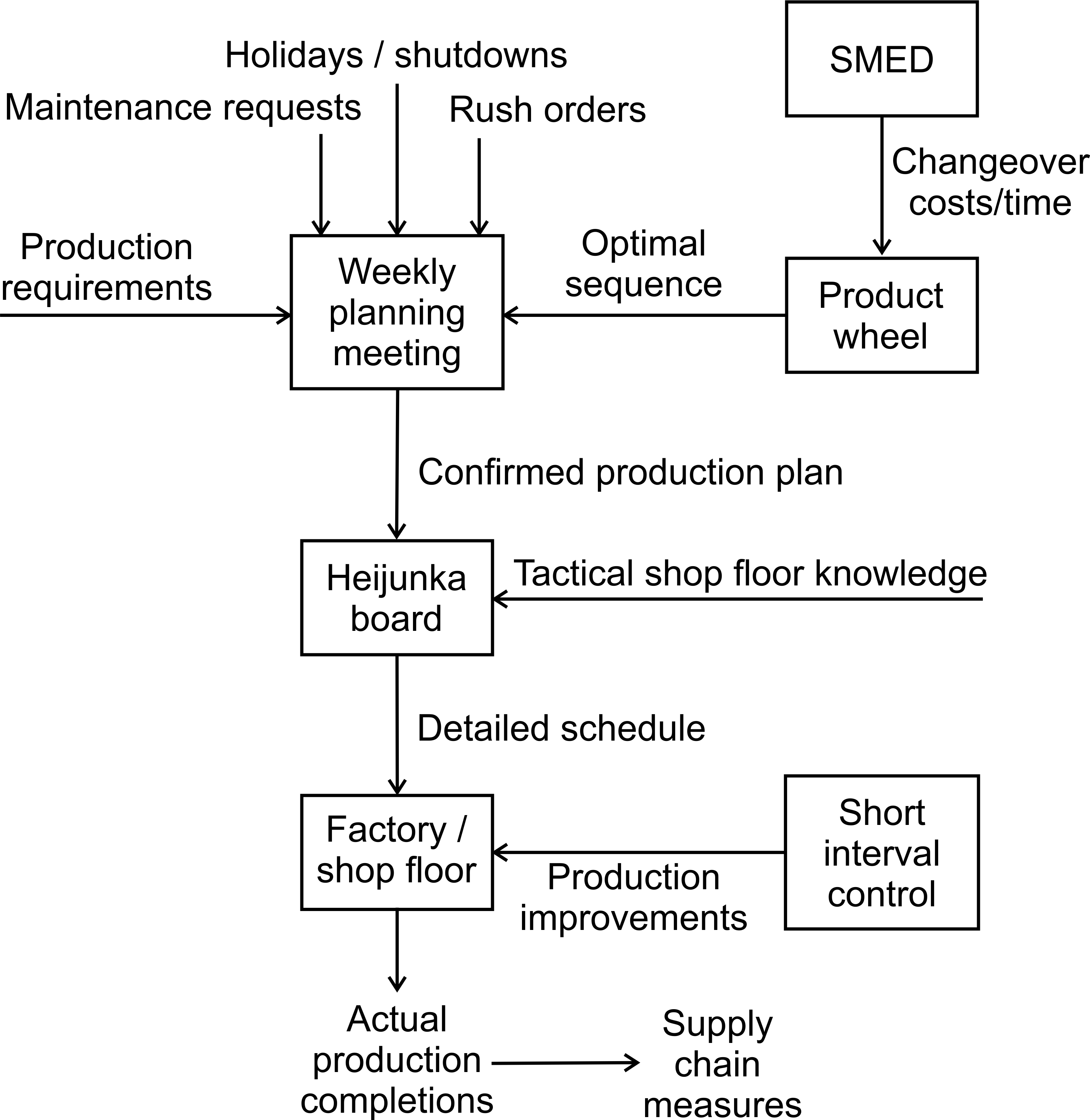
The balanced planning book has set production and distribution targets, determining the quantities of items to be produced and dispatched in each period. The planning book does not care for, or even know when, the items are produced within the period. The next stage of the production planning process, the detailed scheduling, determines the sequence of production within the planning period. This is probably best done in a manual manner-in a weekly planning meeting with the production, engineering, logistics, and the sales/marketing departments – with, or without, the support of production scheduling software. For example, the production department may want to produce items in a particular sequence to minimize changeover costs; engineering may want to schedule some maintenance work; the logistics team know the shipping timetable; and the customer service team know of requests for rush order from customers. This stage also accounts for factors such as national holidays, factory shut-downs, sporting events, and the like.
Hold a weekly planning meeting to consider:
- Downtime requests and maintenance activities.
- Fine tuning the sequence of production to take into account raw material availability, changeover issues not accounted for in the cost/time matrix, breakdowns, etc.
- Urgent requests from customers.
- Overtime requirements.
- Batch sizes and minimum production quantities.
- Truck and container fill.
- Recent run rates and the need to inflate targets to account for predictable yield losses.
- Machine breakdowns and labour availability.
- Recurring quality issues.
- Forthcoming holidays, shutdowns, and sporting events.
There is a considerable amount of Lean advice on detailed scheduling but here is a quick summary of the most important concepts.
5.1 Single minute exchange of dies
The Lean approach advocates reducing the set-up cost/time as much as possible by using the Single Minute Exchange of Dies (SMED) principles of separating out the internal and external activities and reducing their duration and cost, Shingo (1996). SMED allows Lean companies to produce a complete range of products within each replenishment cycle, thus reducing the need to hold cycle stock to cover the time when a product is not being produced. Reaching this state of producing every product every period is the nirvana of Lean production and is known as mix leveling, Ohno (1998).
SMED can reduce the time and cost of changeovers from days down to hours and further down to minutes and seconds. This allows you to produce in small batch sizes. Aim to produce every part in every period. Small batch sizes allow you to get quick feedback on quality issues from downstream processes eliminating the production of large numbers of poor quality products by mistake. Small batch sizes also reduce effective lead-times, allowing both you and your customers to reduce WIP and inventory levels. When your customer learns that you can produce in small batch sizes and deliver quickly and reliably, they start to order more frequently, in small batch sizes, and this has a further smoothing effect on demand.
Single minute exchange of dies
SMED reduces the waste incurred to convert processes from running one part or operation to another. Set-up activities consist of two types of activities: internal activities and external activities. An internal activity is work done while the machine is not producing a good product. An external activity is work done while good products are being produced.
The SMED procedure can be summarized as follows:
Step 1. Separate out the internal tasks from the external tasks. Step 2. Reduce the number and duration of the internal tasks. If this comes at the cost of increasing the number of external tasks, so be it. Step 3. Reduce the external tasks. Step 4. Improve all set-up activities.
A good changeover is a highly choreographed activity, with operators or changeover teams undertaking specific tasks in a highly efficient manner. A slick changeover reduces machine/operator downtime and maximizes the throughput of the system.Despite the popularity of single piece flow and the success of SMED, many industries–especially process industries–do have significant changeover costs and are still driven by large batch sizes. Next, we shall consider how to optimize the sequence of production to minimize the consequences of high changeovers costs via the product wheel.
5.2 Product wheels and changeover times
It is rather rare that products have a dedicated production line. Many products share the same production facilities and changing from one product to the next in the sequence incurs a set-up or changeover cost. This implies that, intermittently, the production line needs to be changed in some manner to allow for a different product to be produced. This set-up or changeover takes time and costs money. If the set-ups are different for each pair of products in a changeover, the question arises–what is the optimal sequence that minimizes the total set-up costs? As all products need to be produced before the end of each replenishment cycle, this is known as a product wheel, King (2009). An example product wheel is illustrated in Figure 5.1.
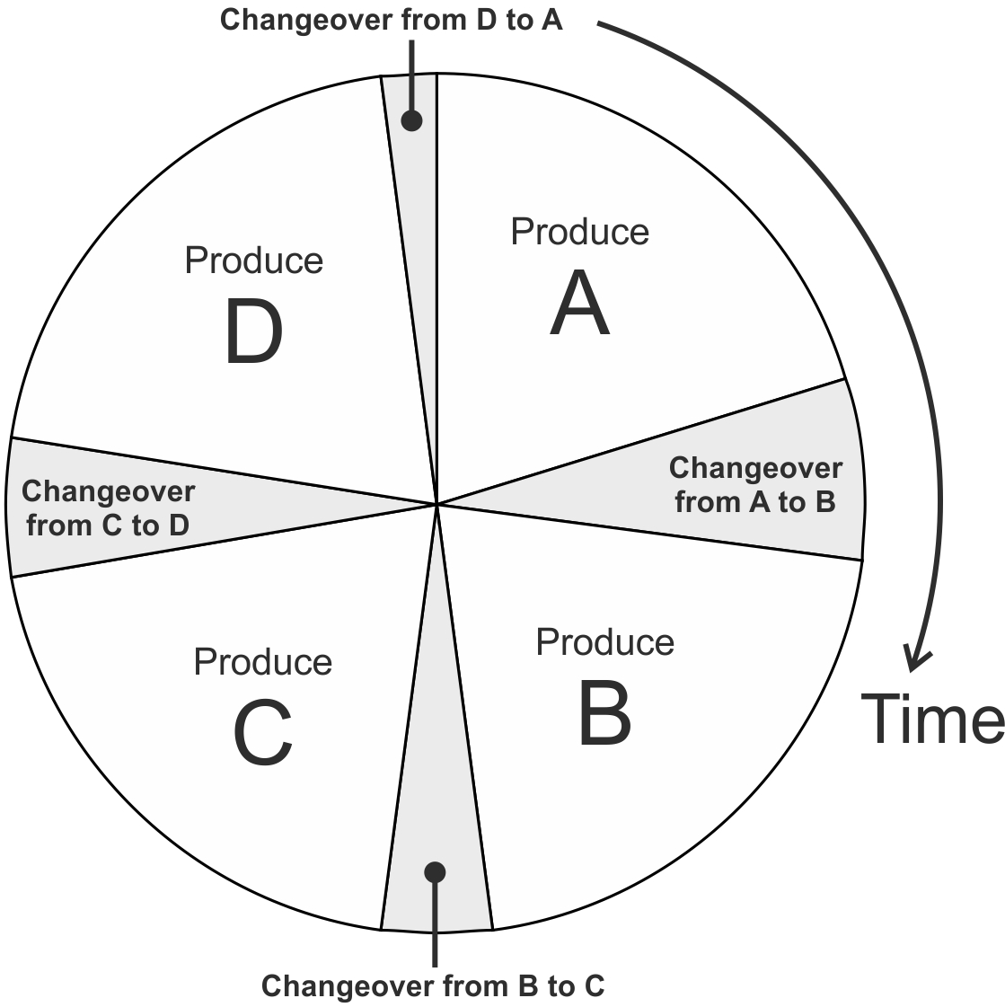
Figure 5.1: The product wheel
Product wheels are a useful tool for minimizing the changeover cost as we cycle through products that share common production facilities. Minimizing the time (or cost) to circumnavigate the product wheel is important even if you already are a SMED expert with slick changeovers. The product wheel is used–not to justify large batch sizes–but to help you minimize batch sizes and their consequences as much as possible. It allows you to cycle through the product range as quickly/cheaply as possible and in some instances it can help you find extra capacity.
Example: Determining the optimal production sequence in the product wheel
In keeping with our spirit of learning by doing approach, let’s see how we can solve the product wheel problem by way of an example.
A company produces fruit drinks. Let us highlight the basic production process of making fruit juice by considering the case of Orange Juice. Oranges are grown in Brazil. In Brazil, the Oranges are squashed, and the juice is distilled into a concentrate. The concentrate is much cheaper to transport than the oranges. The distillation process also separates out the juice from essential oils, and these are stored in separate containers. The orange pulp is also saved and packaged separately to create the orange juice with bits in it later in the process. The three orange components are transported by ship from Brazil to the UK. When the orange concentrate, essential oils, and pulp arrive in the packaging factory, they are combined with water in a big mixing machine. The fruit juice is then put inside a 1-litre TetraPak that is aseptically sealed. The product is then sold as individual 1L boxes or in multi-packs of 6 or 12 1L boxes. Either way, a 1m cube of the product is stacked up on a pallet and distributed to customers. Similar production processes are undertaken for Apple, Pineapple, and Tomato juice.
The production is planned on a weekly basis, each mixing machine producing several different products during the week. Between the production of one product and another, the machine has to be emptied, cleaned and new raw materials piped in. Some products are easier to clean out of the machine than others. For example, apple juice is fairly easy to flush out; tomato juice is harder to remove. So the changeover costs are different as the production line is reconfigured to produce a different product. The TetraPak feeder also has to be changed as the packaging has different designs. Table 5.1 details the changeover cost matrix for the four products.
| Changeover cost | To A) Apple | To B) Orange | To C) Pineapple | To D) Tomato |
|---|---|---|---|---|
| From A) Apple | - | 3 | 3 | 3 |
| From B) Orange | 6 | - | 2 | 4 |
| From C) Pineapple | 9 | 7 | - | 4 |
| From D) Tomato | 12 | 13 | 14 | - |
The four different products \(\{A,B,C,D\}\) can be rearranged into \(4! = 24\) different permutations. However, as after each cycle of the wheel the production sequence is repeated, there are only \(3! = 6\) permutations of interest. In this example, these are: \(\{A,B,C,D,A\},\) \(\{A,B,D,C,A\},\) \(\{A,C,B,D,A\},\) \(\{A,C,D,B,A\},\) \(\{A,D,B,C,A\},\) and \(\{A,D,C,B,A\}\). Notice, here we have returned the wheel to its starting position (arbitrarily chosen to be product \(A\)). These six unique permutations can be represented as a graph with the edges (arrows) representing the changeover cost (or time or other utility) and the vertexes (nodes) representing the products (and, importantly its predecessors), see panel (a) of Figure 5.2.
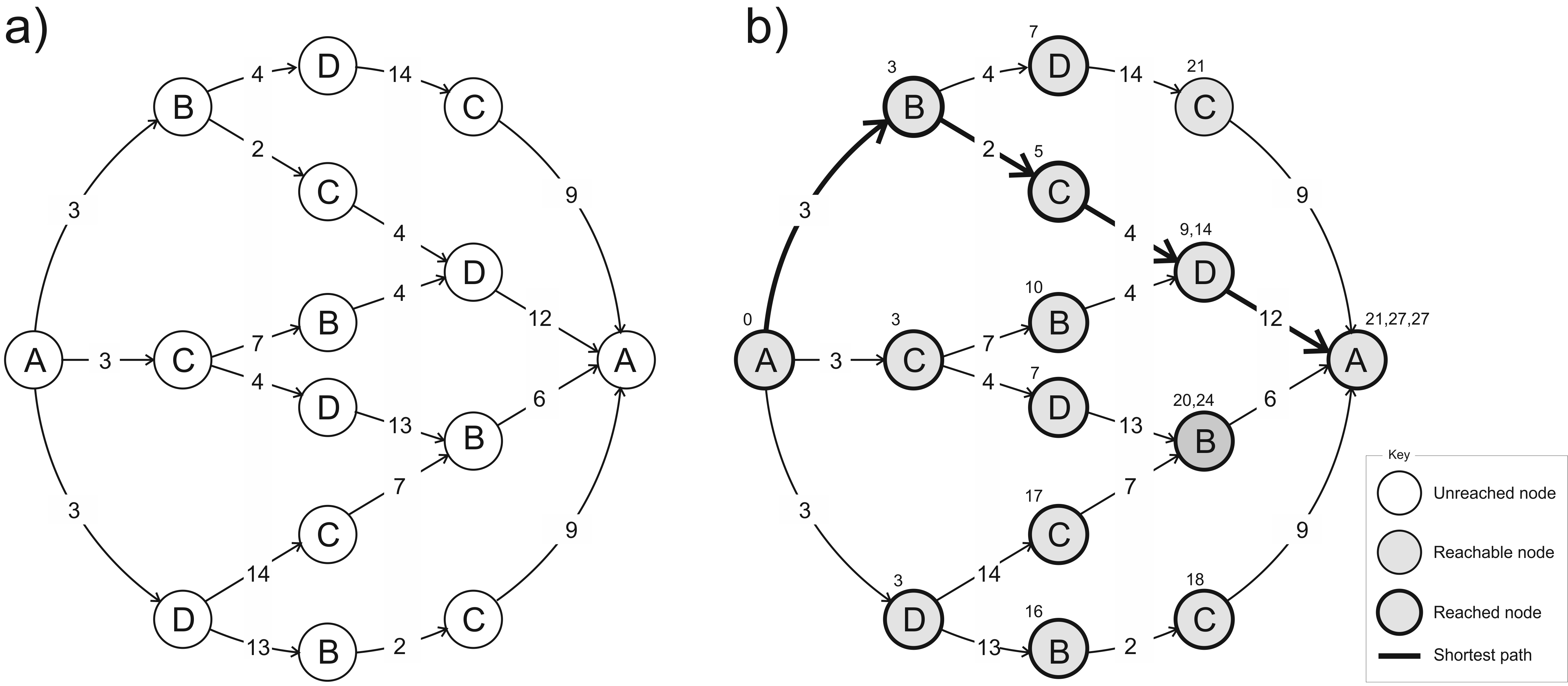
Figure 5.2: The shortest path through the product wheel
The next stage of the analysis is to find the shortest path from \(A\) to \(A\), following the arrows through the graph. The shortest path can be found with the following step-by-step procedure.
Procedure for finding the shortest path in the product wheel
Step 1. Shade all vertices reachable from the current set of reachable nodes.
Step 2. Calculate the cost to reach all reachable nodes.
Step 3. Pick the vertex with the smallest cost and deem it reached (if more than one node has an equal smallest cost, pick one at random).
Step 4. Repeat steps 1-3 until you reach the destination.
Step 5. Determine the shortest path by working backward through the graph looking for the route with the shortest distance.Panel (b) of Figure 5.2(b) shows the output of this procedure. The shortest path has a total changeover cost of 21 and is the shortest path through the product wheel is \(\{A,B,C,D,A\}\).
There are \((p-1)!\) possible solutions with \(p\) products. With two products there is only one route (sequence) through the wheel, three products imply two routes, four products have six possible routes, five products require 24 routes and so on. It is possible to solve this scale of the problem by hand and Appendix D provides the empty graphs required to undertake such a task for easy reference. Notice, the five products problem must be solved as four graphs simultaneously. However, for product wheels of six or more products, the manual approach becomes unwieldy. Fortunately, modern ERP software often has the functionality to solve this problem.
Pop quiz. Table 5.2 provides some example changeover costs in a four product scenario. Using the shortest path algorithm find the optimal sequence of production to minimise the changeover costs in the product wheel. Appendix C.5 provides the answer.
| Changeover cost | To A) Apple | To B) Orange | To C) Pineapple | To D) Tomato |
|---|---|---|---|---|
| From A) Apple | - | 5 | 6 | 10 |
| From B) Orange | 1 | - | 2 | 3 |
| From C) Pineapple | 4 | 5 | - | 9 |
| From D) Tomato | 3 | 6 | 2 | - |
In practice, many companies will not use an algorithm to solve the product wheel. Instead they use intutition or some simple rules of thumb such as going from light colors to dark colors, linking the production cycle to a shipping schedule, or from organic to non-organic products and the like.
5.3 Communicating to production plan to the shop floor
Having forecasted demand, decided on the production quantity, fine-tuned the detailed schedule by finding the optimum sequences through the product wheel, and considered other special factors in a weekly planning meeting, it is now time to communicate the plan to the shop floor. This is often done with a plan that dictates, hour-by-hour, what needs to be produced. Many of the best implementations also allow the shop floor personnel to use their discretion in deciding how the actual production plan is realized based on current tactical knowledge of the shop floor. There are various ways to do this, but here we will describe three common approaches: Heijunka boxes, Gantt charts, and Traffic lights.
5.3.1 Heijunka box
The Heijunka box is a low-tech, low-cost tool to organize and communicate, in a very visual and easy to understand manner, the production plan to the shop floor. It usually consists of a wooden box, or magnetic white board, placed near the pacemaker process, with spaces for each hour of the day and each day of the week. In each of the boxes, a production Kanban can be placed, see Figure 5.3. The production operators at the pacemaker can then simply take the next Kanban out of the Heijunka box when the previous Kanban has been produced. The production workers can manually re-arrange the Heijunka Box to take advantage of the current situation on the production line, for example, if the raw material is not available or a machine has broken down. The timed box also lets operators know whether they are on schedule.
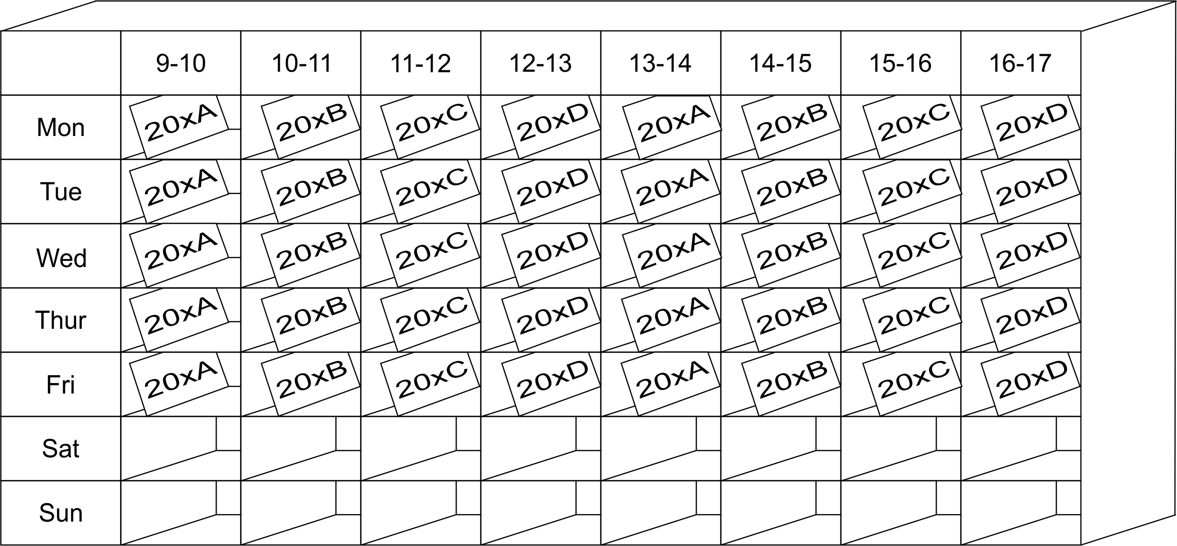
Figure 5.3: Example of a Heijunka Box
5.3.2 Gantt chart
Gantt charts are useful in process orientated industries when changeover costs exist or when there is a selection of different machines or production lines that could be used to realize a production order. Multiple machines/processes are usually represented horizontally, time vertically, as shown in Figure 5.4. Often a vertical bar, representing the current time, moves through the Gantt chart so that one may visually inspect progress against what was planned. This is especially useful when the actual build quantities are plotted in real time with additional bars (the dark gray bars in Figure 5.4) on the Gantt chart. There are process control technologies that can automate this data collection task that can also interface with your ERP system.
There also exists commercial software, either native within your ERP system or externally as a stand-alone system, to automatically schedule orders on the most efficient machines in the correct order to minimize changeover costs/time. The suggested schedule can then be manipulated by dragging and dropping orders around the plan as desired so that one may finesse the schedule, plan maintenance and the like. It is important that information such as the bill of materials, routings, costs, changeover costs and time, production rates, and batch sizes are accurate. This information is likely to change over time, so it needs to be monitored and updated regularly.
For each production run, the first of the two numbers represents the quantity to be produced in the current production run; the second number represents how much of the product is required in the current period. For example, machine 1 will be producing 7000 of the 13500 needed this week, 4750 will be produced on machine 4 and 1750 on machine 5.
The black vertical line represents the current time during the week. The dark grey horizontal bar represents progress made in producing the batch. Machine 1 has has produced more than of the expected quantity to be produced at this time. Machine 2 is behind schedule. The maintenance on machine 3 was completed earlier than expected, and production of product D is ahead of schedule. On machine 5, the production of product D took slightly longer than was planned, the changeover seem to have been done in standard time, but the production of product A started late and machine 5 is behind schedule.
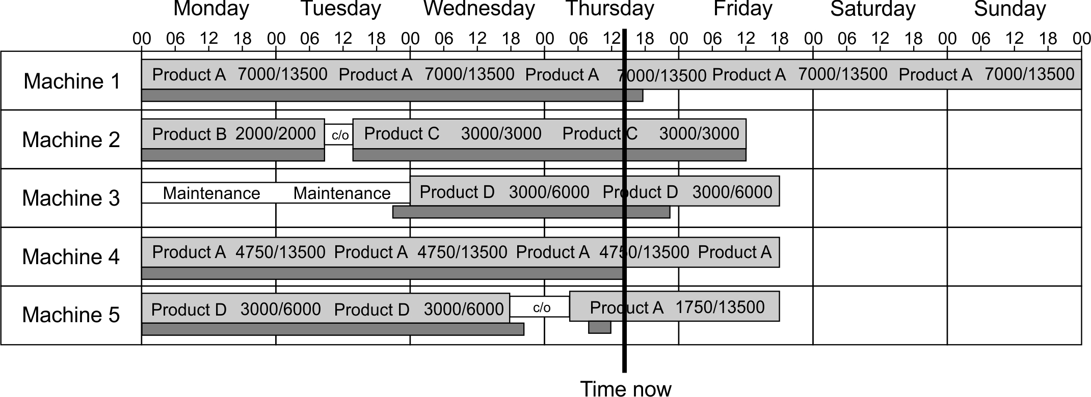
Figure 5.4: Example Gantt chart based Heijunka board
5.3.3 Traffic lights
A traffic light system can also be used to visually communicate production requirements to the shop floor, together with some guidance on the current inventory level versus the safety stock. The production team can then decide for themselves in which order to produce the plan. For example, see Figure 5.5 where 13500 of product A, 2000 of product B, 3000 of product C, and 6000 of product D is required. The colored bars represent the urgency of the production request. The solid black line is the current inventory level. When it is in the green area, then the inventory is above the safety stock target, represented by the boundary between the green and the orange sections. The orange section denotes when the inventory level is below the target safety stock. Red represents an even lower inventory level, an even more urgent situation.
Traffic lights provide a signal to the shop floor about which products should be produced in what order. First, you tackle the items in the red zone, then orange, then green. The traffic light system is useful when the change-over cost/time is either low or constant between items in the product wheel. Furthermore, it gives some autonomy to the shop floor, fostering a sense of empowerment.
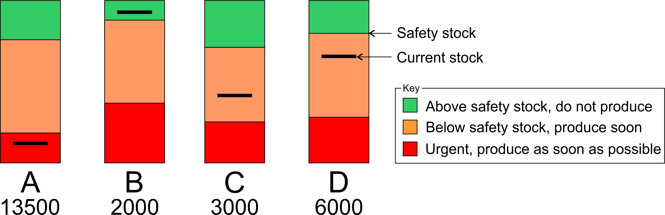
Figure 5.5: Example of a traffic light Heijunka board
5.4 Improving the adherence to plan
Having communicated the firm production plan to the shop floor, the magic of the production system finally happens, and items are manufactured!
What you will quickly realize is that the completed production never quite matches the confirmed production target. Machines will have broken down. Poor quality products may have been produced. Raw material might not be available. The production yield is inconsistent. The production team decides to over-produce in order to run out partly finished batches of raw materials or to avoid a changeover at the end of a shift. Or one of many other root causes mean that actual production differs from target. Over-production results in excess FGI being built-up. Under-production means that you were not able to deliver enough inventory to the customer, potentially impacting service levels and/or creating the need for expedited transportation.
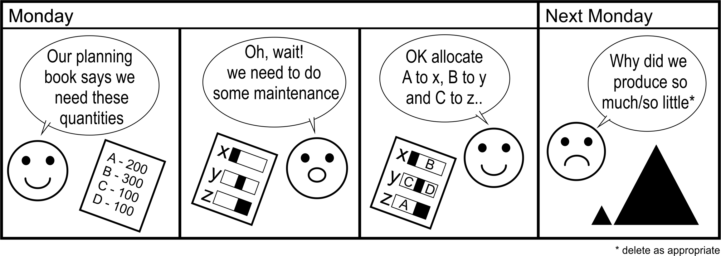
Figure 5.6: Executing the desired plan
You should monitor the adherence to the production plan. Analyze the reasons why you don’t meet the target, either by over- or under-producing. Use an Ishikawa diagram and 5-why analysis to Pareto out the causes of over- and under-production. Identify the root causes and Kaizen those problems out. Use short interval control within each planning period to improve the capability of the production system to adhere to the plan.
Short interval control
Short interval control is a process to improve the effectiveness of production. It involves a team of 3–4 empowered production workers/engineers reviewing the performance of the production system in a 5–10-minute meeting, 3 or 4 times per shift. The following actions are then completed in each of the meetings:
- Review the previous losses (perhaps with the aid of overall equipment effectiveness (OEE). OEE is a way to measure and improve the performance of machines, see Productivity Press Development Team (1999), for more information).
- Assess the effectiveness of previous actions.
- Identify current risks and problems.
- Decide on specific actions; prioritise, allocate resources, set targets.
Train the team to ensure everyone understands the vision. You will need to bring along the people that react cautiously to changes slowly and deliberately. Make sure the team knows that the production plan represents the most cost effective plan for the whole business (and that the safety stock is a target inventory that sometimes we will be above, sometimes below). Remember we have gone through the whole planning procedure to optimize the complete process–not time, nor production cost, nor inventory levels, nor efficiency levels–but the process outputs. Let the planning team focus on creating the production plan and the production team focus on realizing the plan. There is no need, and it often does not help, to let these two functions interfere with each other’s agendas.
Separation of function: Scheduler schedules, production produces
Think of a burger bar. The Chef is responsible for cooking the burger; the Server is responsible for taking the order, receiving the payment and assembling the order with drinks and fries. There is a clear separation of function. The Server is not involved in cooking the burger–the Server tells the Chef what to cook, the Chef prepares it. In your value stream, the production planning team should be responsible for developing the most cost effective production schedule. The production team is responsible for delivering that schedule.5.5 EARS Analysis
Identifying when execution problems exist will be greatly assisted by a review of the most up-to-date Expected–Actual–Recommended–Scheduled production quantities. The Expected quantity, E, is what you would have expected to have produced (at the standard rate) at the current point in time. The Actual quantity, A, is what you have actually produced. Recommended, R, is the quantity that the ERP system recommended that you should produce this week, Scheduled, S, is the quantity that you agreed to build at the start of the week in your production planning meeting. Large differences among these numbers should be examined.
You can use the Expected–Actual–Recommended–Scheduled numbers to determine whether you should cease production early during the current production run because you have been producing at a rate faster than standard, or whether you should extend production beyond the scheduled time because you have produced at a slower rate than expected. During a scheduled production run, the production must be stopped immediately if \(A > max(S,R)\). At the end of the scheduled production run then you may cease production if \(A > min(S,R)\) otherwise you have to consider continuing the production run (and putting your ability to produce other products at risk) or stopping production (and risk of not having enough of the current product).
For example, consider in Figure 5.7. The time from the origin to the vertical dashed line is the allocated production time in the detailed production plan. The expected line gives an indication of the progress that should have been made at all points of time. The expected line meets the scheduled quantity at the end of the allocated production period. In panel A of Figure 5.7, the scheduled production quantity is less than the recommended production quantity (presumably, we scheduled less than the recommended amount to preserve the capacity to produce another product). Also shown in panel A are three possible actual production outputs over time:
Actual production was ahead of expected, and before we reached the end of the production period, we had produced the recommended quantity, at which point we stop producing and move on to the next product in the production plan.
Actual production was ahead of expected, and at the end of the shift, we had produced the scheduled quantity, at which point we stop producing and move on to the next product in the production plan. Note, that we did not stop immediately upon meeting the scheduled quantity, but produced more than the scheduled quantity in an attempt to reach the recommended target.
Actual production could not meet the expected production, and we ended up short of items at the end of the production period. In this case, we must make a decision: either continue producing (and risk not having enough time/capacity to produce the next items in the production plan) or cease production at the end of the shift and move on to the next item (and risk not having enough inventory to satisfy demand).
In panel B of Figure 5.7, the scheduled production was greater than the recommended production (perhaps we wished to build ahead to create some space to conduct maintenance). There are again three different scenarios:
The actual production ran ahead of expected production and production ceased when the schedule production quantity was met.
We ended the production period without actually meeting the scheduled target, but produced more than the recommended target. In this case, we ceased production, as presumably only the recommended quantity was truly required, the scheduled quantity was a wish.
We ended the production period without actually producing the scheduled, or the recommended, quantity. In this case, we should think about whether we continue to produce to make up the shortfall or cease production and move onto the next product in the production plan.
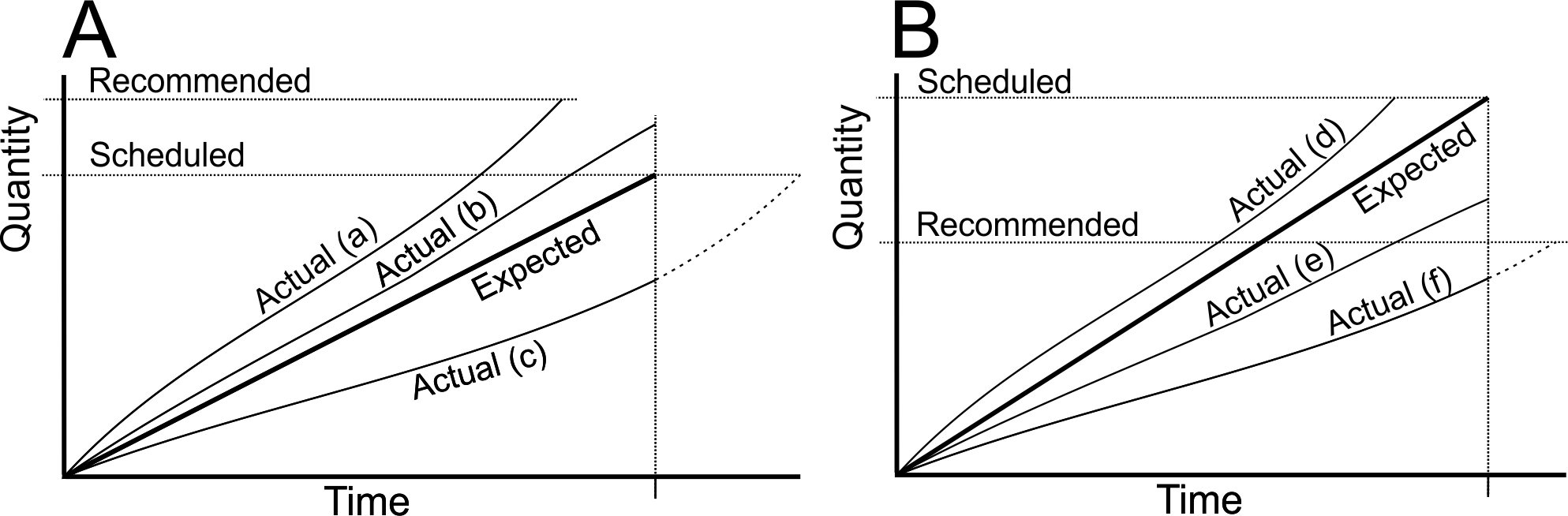
Figure 5.7: Knowing when to stop production with an EARS analysis
Finally, you should measure, and keep a running chart of, your Bullwhip and NSAmp measures. If you suddenly see a sharp increase in these measures, then this is an indication that something has gone wrong and should prompt an investigation. You should collect and measure the Bullwhip and NSAmp performance at two levels.18 The first level is at an aggregate level where you group together all of the products that share the same production facilities. This measure is especially useful for understanding the progress you are making at reducing capacity and Bullwhip related costs. The second level is at an individual item level which is especially useful for managing inventory. The aggregate and the individual measures also give you a roadmap to improve performance; first reduce the aggregate variance measures, then reduce the individual variances.
Having produced the required production, the final chapter considers how one communicates with suppliers to ensure there are adequate raw materials available via the MRP module in your ERP system.
References
Remember, Bullwhip can be measured in at least four different places: the production requirements, the confirmed production, the completed production and the call-off orders sent to the supplier.↩︎