Chapter 2 Strategies for responding to customer demand
Chapter 1 illustrated how to document your supply chain to understand both its structure (the information and material flow) and its dynamic behaviour (via time series analysis). The VSM also identified the pacemaker, the point you schedule in your value stream. The purpose of this chapter is to review a range of replenishment strategies available to set the cadence of your pacemaker. Advice about how to match your replenishment policies to the cost structure in your value stream will then be given.
This workbook is designed to cover make-to-stock (MTS) supply chain settings, and it is particularly useful when: highly variable demand, non-perishable inventory, capital intensive, long lead-time, high-value items, and capacity limitations exist. The approach to creating appropriately smoothed production and distribution targets is a scalable technique that can be used for many products. It creates a volume leveled production plan. Spreadsheets and other manual systems can be used to schedule up to a couple of dozen items. However, ERP and other computerized systems must be used in situations where there are hundreds of products. As most companies have many dozens, if not hundreds of different products, and each product has many raw materials, components, and subassemblies, then an ERP system is often the most useful implementation medium.
2.1 Previous implementations of the techniques in this workbook
It is useful to review some of the real applications that I have been involved with as it highlights the range of situations and potential realizations that a project of this type can take.
Homecare products manufacturer. In this global supply chain, a small number of raw materials were turned into hundreds of SKU’s and sold in many different formats (i.e., various pack sizes, packaging designs, and languages) in many different countries. A simulation model was used to develop management rules for use by the supply chain team. For example, the simulation showed that it was never necessary to ship less than two, or more than three, containers from the Asian supplier to the European manufacturer each week. Requiring the supply chain team to write an exception report and seek management approval for shipments below two containers, or above three, quickly changed their ordering behavior. The process change reduced Muri and Muda; demurrage costs at the ports vanished almost instantly.
Grocery retailer. In this national supply chain, tens of thousands of products are scheduled up to three times a day for delivery to hundreds of stores from dozens of distribution centers. The retailer was concerned about the amount \(Bullwhip\) created between the stores and the distribution centers. Their replenishment system not only amplified the natural weekly cycle in the grocery sales, creating an uneven workload in the distribution centers but also meant that they had to rely on (expensive) third party logistics providers on the peak days to deliver product to stores. This project involved reviewing and adding code to a turnkey IT system responsible for calculating the quantities of products to be sent from DC’s to individual stores. The scale of this project was large, but in many ways, it was an easy project as deliveries were (almost always) received from the supplier on-time and in the right quantities, the data in the existing IT system was of good quality, and the company already had a team of software engineers in place to add code to their computer system.
Consumer electronics group. A global manufacturer sourced raw materials from suppliers located all over the world, often with very long lead-times. A single, capacity limited, manufacturing location produced several dozen intermediate products which shipped to several final assembly sites. Demand was highly variable, and the global shipping lanes of the product had variable lead-times. Initially, a custom-made spreadsheet was used to plan production and distribution. However, later the solution was incorporated into user-defined macros within the company’s ERP system as that allowed for a more efficient workflow and an easier route to widespread adoption in other parts of the organization.
This workbook might not be so useful:
- In make-to-order (MTO) settings which require order book management approaches that we do not consider here.
- When perishable or highly seasonal items are present (this requires forecast or newsvendor-based solutions).
- In job shops, where small volumes dominated by changeover costs call for batch production techniques.
- In settings with intermittent demand, such as spare parts and low demand volume settings.
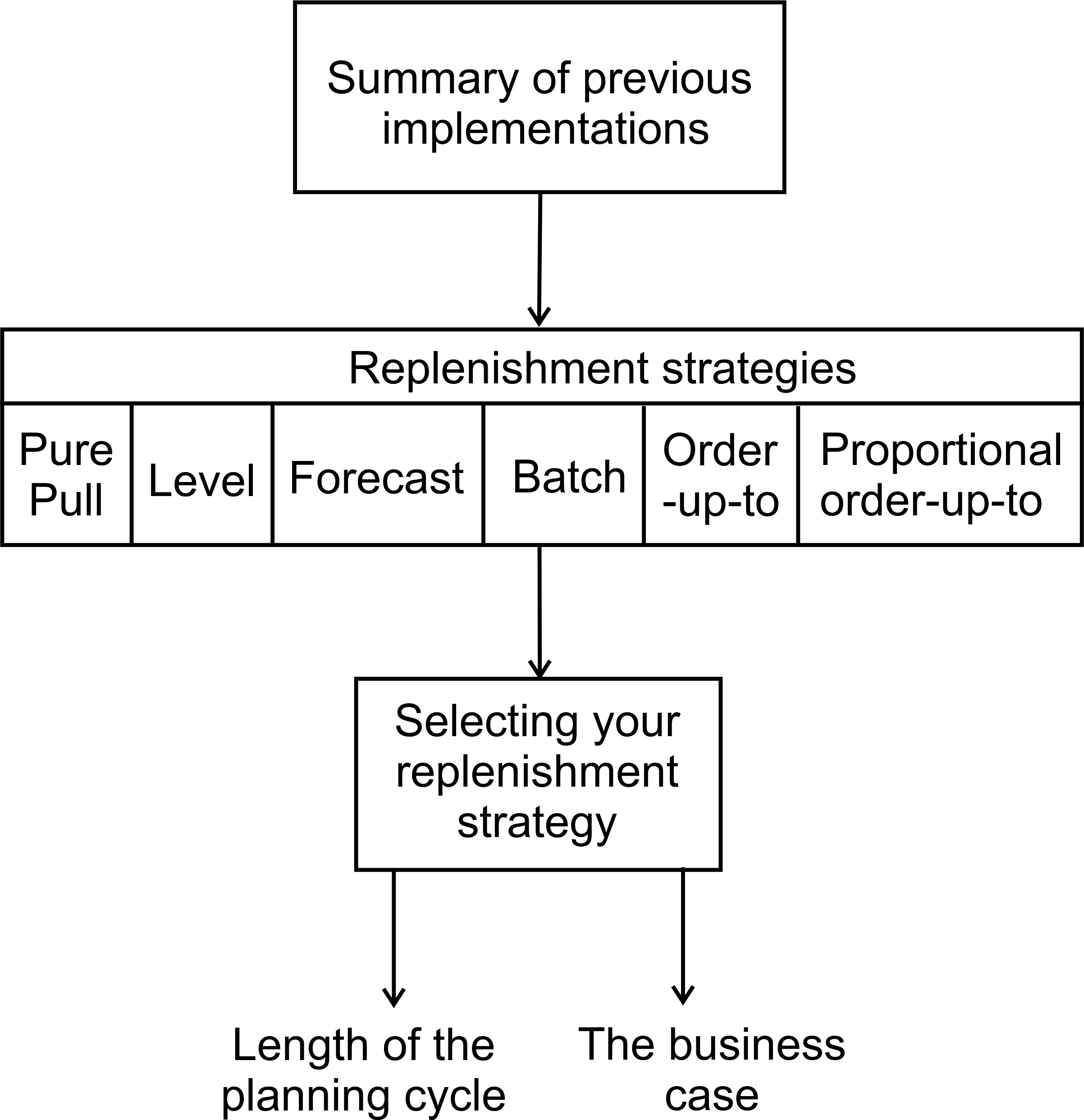
2.2 Selecting your replenishment strategy
Having summarized some implementations and characterized when this workbook is, and is not, useful we proceed to review six different replenishment strategies. Later in the chapter, some guidance on how to select your replenishment strategy will be given.
Figure 2.1, from Towill and Vecchio (1994), provides a caricature of the six primary replenishment strategies for MTS scenarios. For each of the six strategies, demand remains the same, represented here by a sine wave. We can think of the x-axis (not shown to avoid clutter) as time and the y-axis (again not shown to avoid clutter) as the demand quantity. The dynamic, time-based, production/replenishment orders are also represented in Figure 2.1, as well as the inventory behavior associated with each strategy. Let us now review each strategy in turn.
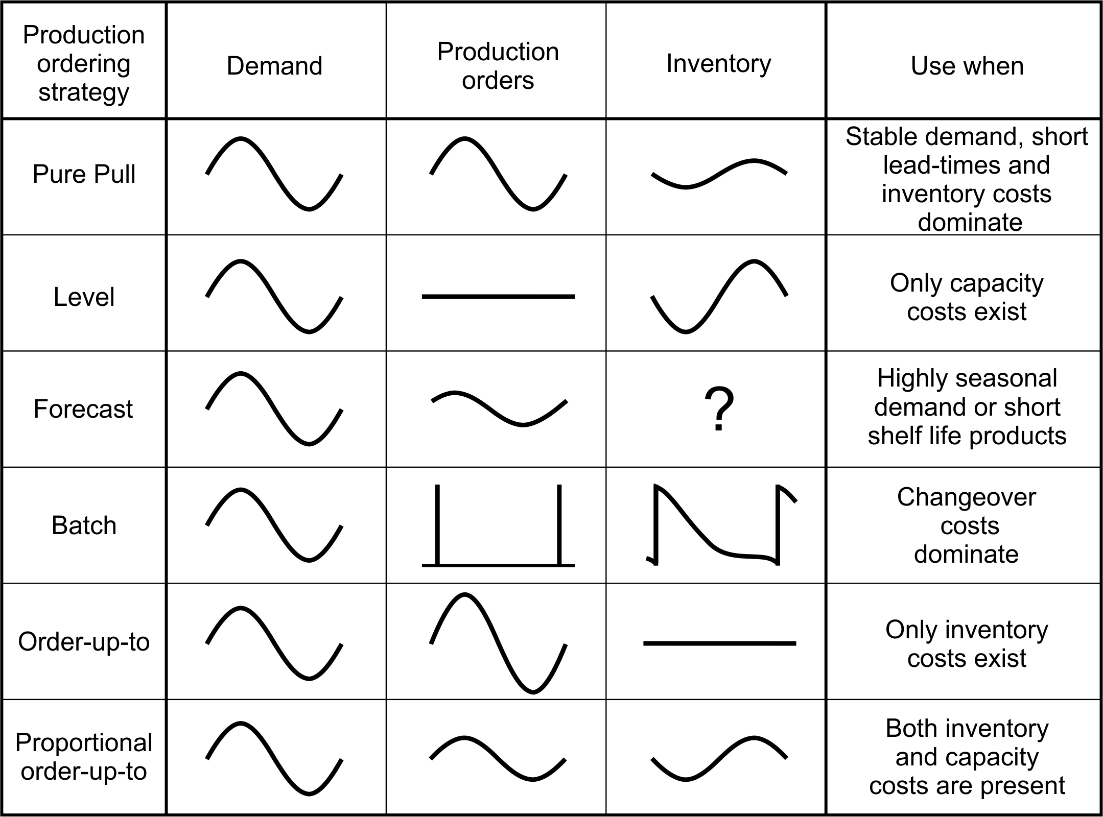
Figure 2.1: Strategies for setting the cadence of the pacemaker
2.2.1 Pure Pull: Producing to customer demand
The Pure Pull strategy sets the production orders equal to customer demand; in this sense, the customer pulls the product through the supply chain. Unfortunately, this means that the demand variability is passed directly onto the production system. The Pure Pull strategy is an easy-to-communicate, easy-to-implement technique (it requires only one piece of information, the current demand), appropriate when lead times are very short, and the demand variability is small. However, demand variability quickly erodes capacity utilization and long lead times increase inventory requirements. As there is no inventory feedback in the policy, when the average demand level drifts higher (lower), the average inventory moves lower (higher). As such, the inventory is uncontrolled. So, despite being a common recommendation, it is a rather questionable strategy with, at best, limited applicability. Despite this, many companies have implemented the Pure Pull strategy and obtained dramatic improvements in their dynamic performance; probably because the previous performance was so poor that even this dubious policy resulted in improved performance. In this sense, the Pure Pull strategy is a step towards removing the Muri and Mura wastes. However, in my opinion, this strategy is not the end of the journey; it is an important first step.
2.2.2 Level Scheduling
Level Scheduling is another approach often advocated in the Lean literature. The basic idea is to produce the same quantity each week, requiring manufacturing to match the production capacity to the required production rate. It attempts to maximize the utilization of production capacity (by creating zero Bullwhip), but the Level Scheduling strategy (like the Pure Pull strategy) leaves the inventory effectively uncontrolled.
Level Scheduling might be a useful strategy in highly automated situations, where investment in production capacity is high, and minimum excess capacity is required. Think of supplying a car assembly plant where the car plant produces the same number of cars every day. In this situation, a co-located supplier can adopt Level Scheduling quite easily. However, if highly variable demand or long lead-times exist, then level scheduling quickly breaks down. The problems originate from having first to identify the average demand, which in many cases changes over time, and then having to absorb all of the demand variability in the inventory levels. If demand has been higher than the average for a few weeks, the inventory levels can be quickly depleted, forcing you to take emergency steps to fortify buffers. If demand is lower than the average for a few weeks, inventory level can build-up, creating the need to cease production to avoid excessive stockpiling.
Companies often try to complement the level scheduling strategy with periodic (say once per month or once per quarter) re-calculations of the level. These re-calculations do little to improve inventory control, and the policy quickly degenerates into almost constant manual adjustments.
2.2.3 Forecast
The Forecast strategy is useful when demand is (a) highly seasonal (for example, annual flowering plants or fashionable ski-wear), or (b) where the product life cycle is very short (croissants or newspapers, for instance). In case (a), the inventory can be pre-produced before the selling season, but once the selling season is over, the goods become unsellable. In case (b), there is no opportunity to hold inventory as nobody wants to buy spoiled food or yesterday’s newspaper. In both cases, we must forecast demand, produce and ship to the forecast, and hope for the best.
If our forecasts were optimistic (i.e. too high), we would be left with unsold inventory. In some cases, this unsold inventory can be recycled or reused in some way (recycling newspapers, selling last season’s fashion items into a secondary market, leaving annual flowering plants to seed to create next year’s crop). If our forecast was too pessimistic, then some demand existed that could not be satisfied; unforgiving customers may defect to competitors (potentially forgoing the net present value of all future cash flows).
This type of problem requires a newsvendor analysis. The input data is some forecast of the demand distribution and the expected over- and under-age costs. The output of the newsvendor analysis is a production quantity that balances the over- and under-age costs to produce a minimum total expected cost solution.
2.2.4 Batch
The Batch policy is relevant in low volume, high set-up cost settings where one production run will satisfy demand over many periods. In this case, we incur a set-up cost to produce a batch of product. Much of the batch is not required immediately but transferred into inventory and used to satisfy demand in the future. The inventory levels are monitored, and when inventory is sufficiently low, a new batch is ordered or produced.
While batching creates substantial Bullwhip and NSAmp, it is unavoidable in some situations. Consider the case when the production process was designed for the high volume stage of a product’s lifecycle and, at the end of the life, the low demand volume does not warrant further investment in a new/different production process. However, 20% of your products will create 80% of your bullwhip problems. The products produced in Batch mode are typically low volume items and usually do not take up a large proportion of the available capacity. If Bullwhip can be eliminated for the high volume items, time in the production schedule can be made for the low volume items produced in Batch mode.
The actual size of the batch, \(Q\), can be determined by many different approaches. In a purchasing environment where all of the required order effectively arrives at once, the economic order quantity (EOQ) formula (or some variant of it) can be used to balance the set-up and inventory holding costs. The economic production quantity (EPQ) formula is useful in production settings when the required batch arrives, slowly over time.
2.2.5 Order-up-to policy
The Pure Pull, Level and Forecast replenishment strategies have no inventory feedback control. The Batch policy has a primitive feedback loop–the inventory levels are monitored, and when the inventory level falls to a certain point, a new batch is produced. However, this is more of an off-line feedback loop, that creates a bang-bang type of control. Proper inventory control requires inventory and work-in-progress (WIP) feedback control. That is, the actual inventory (and WIP) level needs to be monitored, compared to the target inventory (and target WIP) and the difference accounted for in the replenishment quantity.
The order-up-to (OUT) replenishment algorithm is a well-established replenishment algorithm that possesses these inventory and WIP feedback loops. The OUT policy requires a forecast of the demand during the lead time and the review period. It also monitors and adjusts for deviations in the inventory levels and WIP levels from a target. In this way, it maintains control over the inventory and WIP levels. The OUT policy is known to be an optimal policy (it is the best linear policy among all policies that could exist) for minimizing inventory levels in a single echelon of a supply chain.
The OUT policy is also present native in many ERP systems, making it a popular choice to control high volume, regularly produced, items when inventory costs dominate. While the OUT policy can cope with both variable demand and long lead-times, it always creates Bullwhip when exponential smoothing or Holt’s method is used to forecast demand, for all possible demand patterns and all lead-times (see Dejonckheere et al. (2003) and Li, Disney, and Gaalman (2014)). It is also very sensitive to errors in the lead-time. For example, the OUT policy requires information of the lead-time when determining the forecast of demand over the lead time and review period. If this lead-time is different from the actual physical lead-time, the OUT policy does not work well and can create chaos in supply chains (Wang, Disney, and Wang (2012)). However, if the lead-time information is correct, the OUT policy does well at managing inventory.
Managing supply chains is a bit like taking a hot shower. When in a shower we want to match the temperature of the water to what we find comfortable. In a supply chain, we want to match supply with demand. There is a lead time between the action (turning the tap, setting production/distribution targets) and the consequence (the temperature of the water falling on our head, receiving the production/deliveries). In the shower, if we turn the tap(s) to quickly the water temperature bounces between the extremes of too cold and too hot, see Figure 2.2. This analogy is a fair representation of an OUT controlled supply chain. The OUT policy reacts very quickly to deviations from targets. Next, we will consider a modification to the OUT policy where we turn the taps slowly to match supply with demand. This modified policy is known as the proportional order-up-to (POUT) policy.
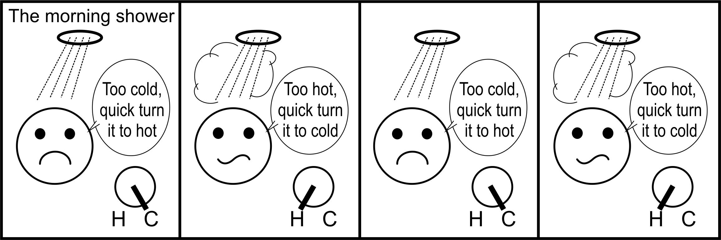
Figure 2.2: Turning taps too quickly in the shower means you don’t get the right temperature
2.2.6 Proportional order-up-to policy (POUT)
The POUT policy is very similar to the OUT policy. It contains just one more parameter, a parameter that regulates how fast the system responds to deviations from target inventory and WIP positions. The variable demand and forecast errors of that demand over the lead-time and review period cause these deviations. The POUT policy is easily incorporated into spreadsheets, in-house software, and ERP systems. All that is required is to change one calculation by adding one variable into the OUT policy. This additional variable \(\beta\) is a proportional feedback controller.
Let’s consider the shower analogy a little bit more. We all know the trick to getting the temperature right in the show is to turn the taps slowly, just a little, and to wait for the water to go through the pipe before making further adjustments. We must do the same in a supply chain; we should react slowly to the discrepancy between the target and actual inventory and WIP levels by using a proportional feedback controller, \(0\leq 1/T_i<2\). In this way, the supply chain avoids oscillating between the extremes of producing large amounts, followed by periods of low (or no) production. The \(T_i\) parameter regulates how fast the supply chain reacts to changes in the demand pattern; in the shower analogy, \(T_1\), is the speed at which we turn the taps.
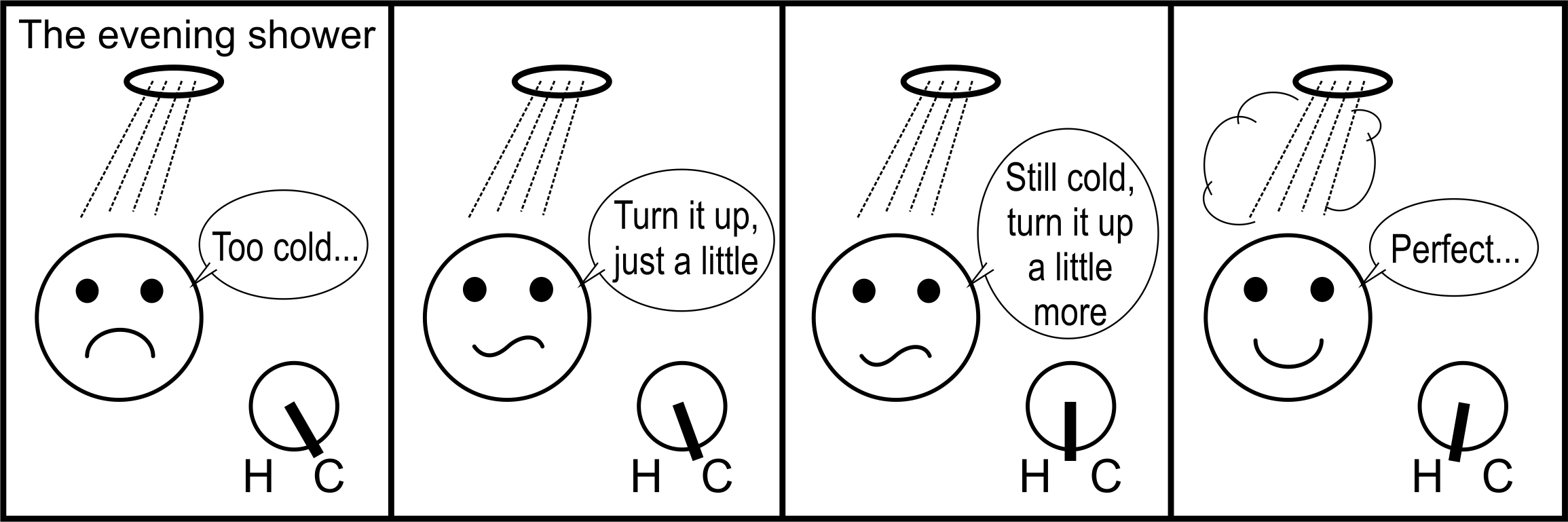
Figure 2.3: To get the right shower temperature, you turn the taps slowly
Under constant lead-times, the POUT policy increases inventory variability but reduces capacity costs and the bullwhip effect and is robust to lead-time errors. In a stochastic lead-time setting, the POUT outperforms the OUT policy with reduced inventory variability and reduced capacity costs. The POUT policy is also robust to errors in the lead-time information as well as stochastic lead-times. In a multi-echelon supply chain setting, total supply chain costs are minimized with the POUT policy (as the upstream player inventory and capacity costs are reduced more than the upstream player’s inventory costs increase). The POUT policy also contains the OUT policy as a particular case (when \(T_i = 1\)). If you are in a capital intensive or a capacity limited setting, the POUT is essential.
2.3 Which replenishment strategy is best for you?
Figure 2.1 highlights that there are six main replenishment strategies available for setting the cadence of your pacemaker.
 A Shiny App is available here where you can explore the dynamics of the six different replenishement strategies in Figure 2.1 interactively.
Which strategy is (or strategies are) the most suitable for you? Well, it depends on context and costs. Also, perhaps one part of your business (product) requires one strategy, and another part (product) requires a different one. Your strategy choice may also change over a product’s life cycle or change as your capability and confidence develop. Table 2.1 summarizes the issues and benefits of each replenishment strategy, highlighting when each approach may be useful.
| Strategy | Benefits | Issues | Useful when |
|---|---|---|---|
| Pure pull. Produce to the current demand rate (from either the next echelon or from the end consumer). | Easy to communicate and implement. | No inventory feedback is present, so inventory levels are uncontrolled. Demand variability hits the shop floor directly. | Your customer is willing to wait for your product, or lead-time is very short. Demand has no trends and has little variability. High-volume demand is produced every period. Capacity, inventory, & backlogs have no cost. |
| Level Produce to average demand (with or without periodic changes in the safety stocks or number of Kanbans). | Easy to communicate and implement. If capacity equals average demand, capacity is fully utilized. | No inventory feedback is present, so inventory levels are uncontrolled. No trends in demand are detected. The periodically changing safety stocks add demand shocks. | Demand has no trends and has little variability. High-volume demand produced every period. Inventory & backlogs have no cost. Capacity is costly. Lead-times are short. |
| Forecast Produce to a forecast. | Easy to communicate and implement. Some balance between capacity and inventory is achieved. | No inventory feedback is present, so inventory levels are uncontrolled. Trends in demand are forecasted but, due to the lead-time, the average inventory levels do not converge to the safety stock target. | Demand has no trends & has little variability. High-volume demand produced every period. Capacity, inventory & backlogs have costs. Lead-times are short. |
| Batch MTO/EOQ: Produce a minimum campaign size. | Can cope with variable lead-times. Minimizes the sum of set-up & inventory holding costs. | Produces a lot of Bullwhip, but usually small volume with little impact on the availability of capacity. | For low volume products only made intermittently. Lead-times are short or long. |
| Order-Up-To Produce to a forecast and account fully for inventory and WIP discrepancies. | Inventory & WIP levels are controlled. Inventory & backlog costs are minimized. Available native in many ERP systems. | This system will almost always produce Bullwhip for all demand patterns & all lead-times. The system will become chaotic when the lead-times are incorrectly specified. | Demand has trends but has little variability. High-volume demand produced every period. Capacity has no cost, only inventory and backlog costs are present. Lead-times are short or long. |
| Proportional Order-Up-To Produce to a forecast and account for inventory and WIP discrepancies only fractionally. | Can cope with variable lead-times and trends in demand. Always able to eliminate Bullwhip. Inventory & WIP levels are controlled. | Requires a change to most ERP systems via a user-defined macro or custom coding of bespoke systems. Difficult to communicate. Policy requires an extra parameter. | High-volume demand produced every period. Capacity, inventory & backlogs have costs. Lead-times are short or long. |
Table 2.2 lists some questions that you should think about when selecting your replenishment strategy. The answers will guide your choice, see Appendix C. You will need to identify the right strategy for each product/customer pairing, but after considering a few products in each of the major categories in your business, you will be able to come up with a limited number of strategies that work for you.
| Question | Yes | No | |
|---|---|---|---|
| 1 | Our inventory is expensive and/or we hold a lot of it. | \(\square\) | \(\square\) |
| 2 | We regularly work overtime to meet peak production targets and then stand idle in periods of low demand. | \(\square\) | \(\square\) |
| 3 | We have high capacity costs. | \(\square\) | \(\square\) |
| 4 | We have high changeover costs, or changeovers are of a long duration. | \(\square\) | \(\square\) |
| 5 | We are capacity limited. | \(\square\) | \(\square\) |
| 6 | We suffer from low availability and/or low fill rates. | \(\square\) | \(\square\) |
| 7 | We regularly use sub-contractors to meet peak demands. | \(\square\) | \(\square\) |
| 8 | We often use expedited transport modes and/or air freight to avoid stock-outs. | \(\square\) | \(\square\) |
| 9 | The cost of not having stock available is high. | \(\square\) | \(\square\) |
| 10 | We have long lead-times. | \(\square\) | \(\square\) |
| 11 | Our demand is tough to predict accurately. | \(\square\) | \(\square\) |
| 12 | Our process is not very capable. We regularly under- or over-produce to our production target. | \(\square\) | \(\square\) |
| 13 | We have significant amounts of production WIP and/or goods in transit. | \(\square\) | \(\square\) |
| 14 | We experience excessive volatility in demand and/or production orders. | \(\square\) | \(\square\) |
| 15 | Our inventory levels fluctuate widely. | \(\square\) | \(\square\) |
| 16 | Our lead-times are highly variable. | \(\square\) | \(\square\) |
| 17 | The demand volume is high, or we produce the product every week. | \(\square\) | \(\square\) |
| 18 | Our selling season, or the shelf life of our product, is very short. | \(\square\) | \(\square\) |
2.4 Determining the length of the planning cycle in your value stream
Another important decision, if you have the luxury of being able to change it, is the length of the planning cycle. For example, are you planning on a daily, weekly, or monthly basis? In many settings and industries, this is a given. However, if you could specify the cycle length and you wished to minimize inventory costs alone, then you should make your planning cycle as short as possible. Short planning cycles are possible if your customer is nearby (so that you can afford to make frequent deliveries) and the demand is relatively stable (so that you don’t create too much Muri). However, if your customer is six weeks away via a global shipping route and the ship only sails once per week, there is little point in re-planning your supply chain every day. Instead, you should match the length of your production planning periods to the frequency of the shipping schedule. Aggregating multiple days of demand into one plan also creates a temporal pooling effect–the aggregation permits the variable daily demand to be spread out over time, allowing you to produce a smoothed average daily demand quantity over the planning period–helping you to avoid unnecessary Muri.
Under the OUT policy (and the Pure Pull policy) there is a natural balance in the optimal length of the planning cycle. Inventory costs are minimized by rescheduling every day (or even more frequently), while capacity costs are reduced by rescheduling as infrequently as possible. Somewhere in between, there will be a rescheduling frequency that minimizes the sum of these two costs. The OUT policy, however, is never able to out-perform a properly designed POUT policy. There is also a natural sequence to implement the POUT policy. We should first implement the POUT policy and then shorten the length of the planning cycle. If we shorten the planning cycle first, without production smoothing via the POUT policy, we can fall into a capacity utilization trap. The short planning cycle without proper proportional feedback control amplifies the Bullwhip effect, leading to the wastes of Muri and Mura (Hedenstierna and Disney (2018)).
Finally, although it is a difficult idea to sell, collecting the overtime/idling requirements to the beginning of the planning cycle allows one to reduce the effective lead-time. This is especially beneficial when you plan production every week, but make deliveries to your customer every day. This may mean that you schedule production on Fridays, identifying and completing any expected overtime requirements in the forthcoming weekend and curtailing unwanted production on Mondays.
2.5 The business case
Solving the Bullwhip problem and reducing your Mura and Muri will have a profound effect on your Lean journey. You will find it easier to identify, remove (and keep removed) Muda, by tackling Mura and Muri–the last remaining sources of waste in many organizations. However, this is not a small project and not one that is likely to be completed by a single person.
The cost of the project. Conservative estimates of the effort involved in a project such as this are about two plus person-years of work. However, many people will need to participate in the project as access to specialist skills are required: IT, ERP, supply chain, production planning, inventory management, production, engineering, etc. Management will also need to offer their support and staff will have to buy-in to the changes, both of which will require time. Many of the changes that occur in a project such as this play out over a long time, across different departments and businesses, and often over a wide geographical area. It will take time to understand current performance, implement the required changes, and observe the impact. You will need to be patient and persistent.
Benefits. Ultimately, the utilization of your capacity and inventory will be optimized, reducing inventory and capacity costs. You will be able to demonstrate improvements in supply chain performance measures such as availability, fill rates, shortages, NSAmp, and Bullwhip. There will also be a reduction in operating expenses and costs such as overtime, and expedited transport. These factors are easily monitored, predicted, and quantified. However, many of the benefits will be intangible, unmeasurable, or unquantifiable. For example, workers will experience a better, more predictable work-life balance, leading to less staff turnover and reduced hiring, firing and training costs. Increased staff retention leads to higher quality and productivity. The planning, production, and logistics activities will be less chaotic. You will have streamlined your planning processes into one system, rather than being done in a multitude of spreadsheets by many different people and departments all over the organization and possibly throughout your supply chain. There will be one set of information that you will be working from, improving the data accuracy and visibility of your supply chain. The nature of conversations held will change, from questioning the correctness of the data and why decisions were made, to deciding how to achieve the desired plan and how to cope with unforeseen circumstances.
Costs that can be reduced when eliminating Muri and Mura
- Over-time, idling and subcontracting as you increase your capacity utilization.
- Expedited transportation.
- Firing, hiring, and training costs.
- Intangible costs associated with a poor work/life balance.
- Back-order costs as you will have better supply chain visibility.
- Inventory costs, as you will have a more responsive production system.
- Bullwhip costs associated with labor utilization and opportunity costs associated with the use of expensive capacity.
Dynamically designing your replenishment strategy is also an educational journey. You will be using logical reasoning, maths, and the scientific process to create a balanced and considered action plan for your company. You will be able to defend your decisions based on facts and information within a well-designed system, rather than reacting to your environment with emotion and panic. You will have the satisfaction of executing the best process, achieving best practice, and obtaining the best performance. The more efficient planning process will allow the planning team to focus more on higher value-adding work.
This chapter has reviewed a range of replenishment strategies and provided a means to select an appropriate strategy for your value stream. All replenishment strategies require some sort of forecast; this is the subject of the next chapter.