D The standard normal distribution
As we have seen the normal distribution plays an important role is setting safety stock and capacity levels. The standard normal distribution has a mean of zero and a unit standard deviation. In this Appendix we review some of its basic properties.
 A Shiny App is available here where we can explore the normal distribution interactively. The App is able to calculate and plot the probability density function, the cumulative density function, the loss function, and their inverses.
D.1 Probability density function (pdf) of the standard normal distribution
\(\varphi[u]\) is the probability density function for the standard normal distribution. Here \(u\) is the standard normal random variable, \(-\infty<u<\infty\), \(u \in \mathbb{R}\). Mathematically it is given by,
\[\begin{align} \varphi[u]=\underbrace{\frac{1}{\sqrt{2\pi}}\text{exp}\left[-\frac{u^2}{2}\right]}_{\text{Mathematically}}=\underbrace{\text{NORMDIST(}u\text{,0,1,FALSE)}}_{\text{In Excel}}=\underbrace{\varphi[u]: u\rightarrow z}_{\text{From Look-up Table}}, \tag{D.1} \end{align}\]
where “\(\varphi[u]:u\rightarrow z\)” means that the \(u\) is replaced with \(z\) in the look-up table that is available here. \(\forall u, \varphi[u]>0\). \(\varphi[u]\) is concave between \(-1<u<1\) and convex when \(u<-1\) and when \(u>1\); this relationship leads to the definition of the standard deviation. The inverse relationship for \(\varphi[u]\), \(\varphi^{-1}[u]\) is
\[\begin{align} \varphi^{-1}[u]=\underbrace{\pm i \sqrt{\text{Log}[2\pi]+2\text{Log}[u]}}_{\text{Mathematically}}=\underbrace{\pm \text{SQRT(ABS(LN(2* PI())+2 *LN(}u)))}_{\text{In Excel}}, \tag{D.2} \end{align}\]
Figure D.1 provides a visualization of the standard normal distribution.
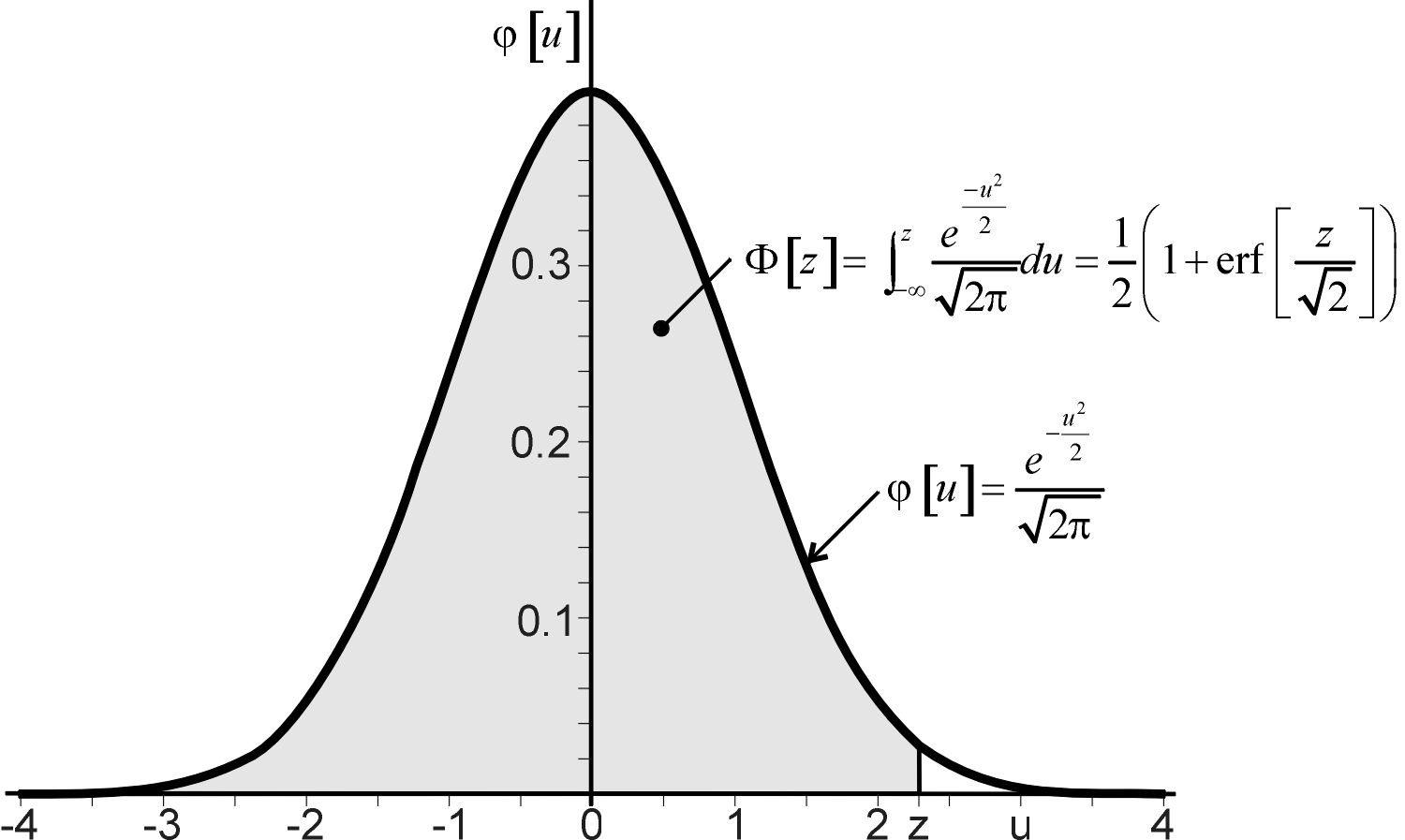
Figure D.1: The standard normal distribution
D.2 Cumulative probability density function (cdf) of the standard normal distribution
\(\Phi[z]\) is the cumulative probability density function (cdf) for the normal distribution,
\[\begin{align} \Phi[z]=&\underbrace{\int^z_{-\infty}\phi[x]dx=\frac{1}{\sqrt{2 \pi}}\int^z_{-\infty}\text{exp}\left[-\frac{x^2}{2}\right]dx}_{\text{Conceptually}}=\underbrace{\frac{1}{2}(1+\text{erf}\left[\frac{z}{\sqrt{2}}\right])}_{\text{Mathematically}}\\ =&\underbrace{\text{NORMDIST(}z\text{,0,1,TRUE).}}_{\text{In Excel}} \tag{D.3} \end{align}\]
The inverse cdf of the normal distribution, \(\Phi^{-1}[z]\) is given by
\[\begin{align} \Phi^{-1}[z]=\underbrace{\sqrt{2}\text{erf}^{-1}[2z-1]}_{\text{Mathematically}}=\underbrace{\text{NORMSINV(}z)}_{\text{In Excel}}. \tag{D.4} \end{align}\]
\(\Phi[z]\) is an increasing function within the interval \(0<\Phi[z]<1\) for $-<z<}. The Error function, \(\text{erf}[z]\), is given by
\[\begin{align} \text{erf}[z]=\underbrace{2\Phi[z\sqrt{2}]-1}_{\text{Mathematically}}=\underbrace{\text{ERF(}z).}_{\text{In Excel}} \tag{D.5} \end{align}\]
Both \(\Phi[z]\) and \(\text{erf[z]}\) cannot be expressed in terms of finite additions, subtractions, multiplications and root extractions. So both must be either computed numerically or otherwise approximated, Weisstein (2012). Figure D.2 illustrates the cumulative distribution function of the standard normal distribution.
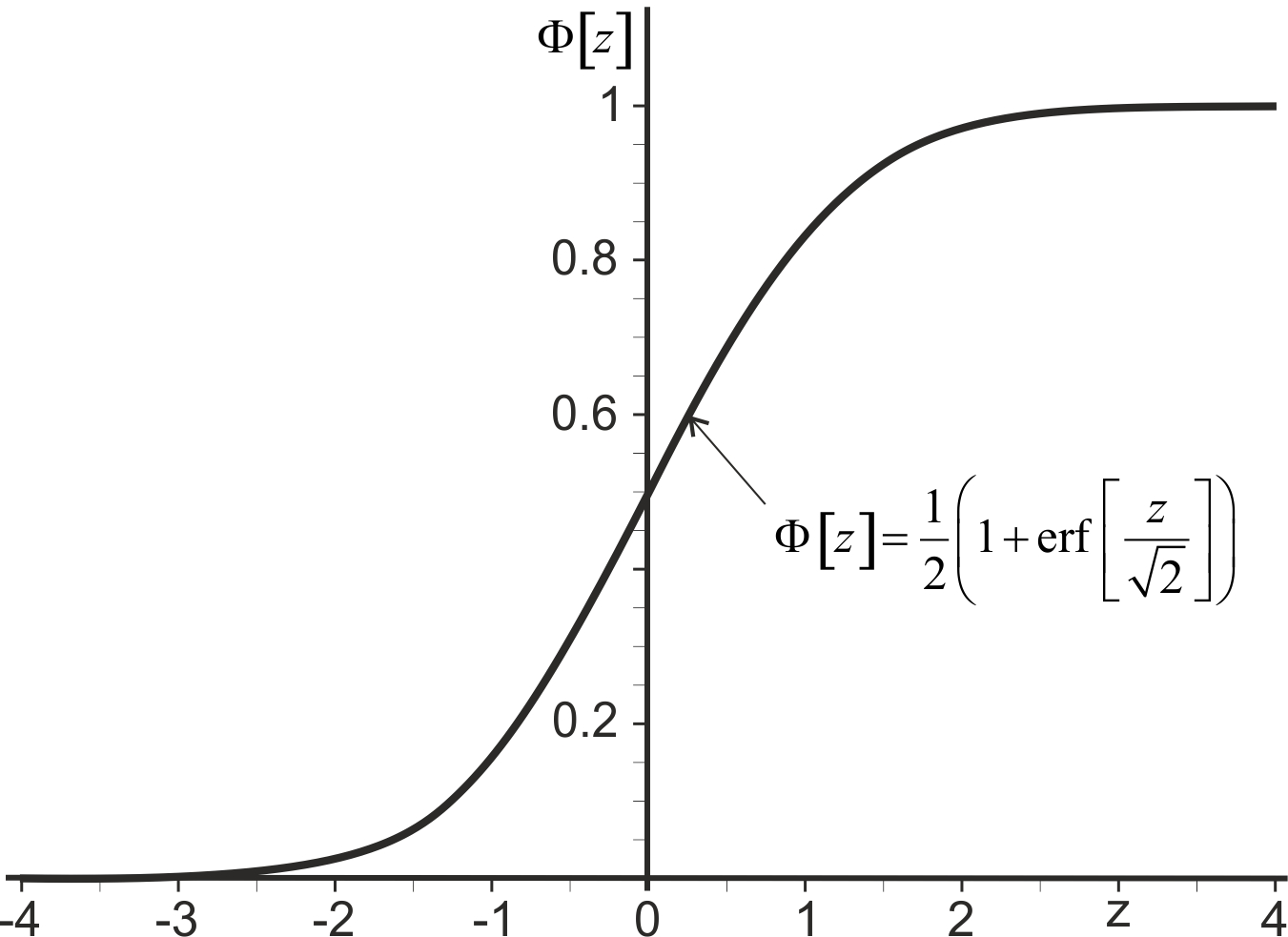
Figure D.2: The cumulative distribution function of the standard normal distribution
D.3 The loss function of the standard normal distribution
The loss function of the standard normal distribution, \(L[z]\), is defined by
\[\begin{align} L[z]=&\underbrace{\int_z^\infty \varphi[x](x-z)dx=\int_z^\infty (1-\Phi[x])dx}_{\text{Conceptually}}\\ =&\underbrace{\frac{1}{\sqrt{2\pi}}\text{exp}\left[-\frac{z^2}{2}\right]-\frac{z}{2}\left(1-\text{erf}\left[\frac{z}{\sqrt{2}}\right]\right)}_{\text{Mathematically}}= \underbrace{\varphi[z]-z(1-\Phi[z])}_{\text{Via Look-up Table}}\\ =&\underbrace{\text{NORMDIST(}z\text{,0,1,FALSE)}-z\times\text{(1-NORMDIST(}z\text{,0,1,TRUE))}.}_{\text{In Excel}} \tag{D.6} \end{align}\]
Figure D.3 illustrates the Loss function.
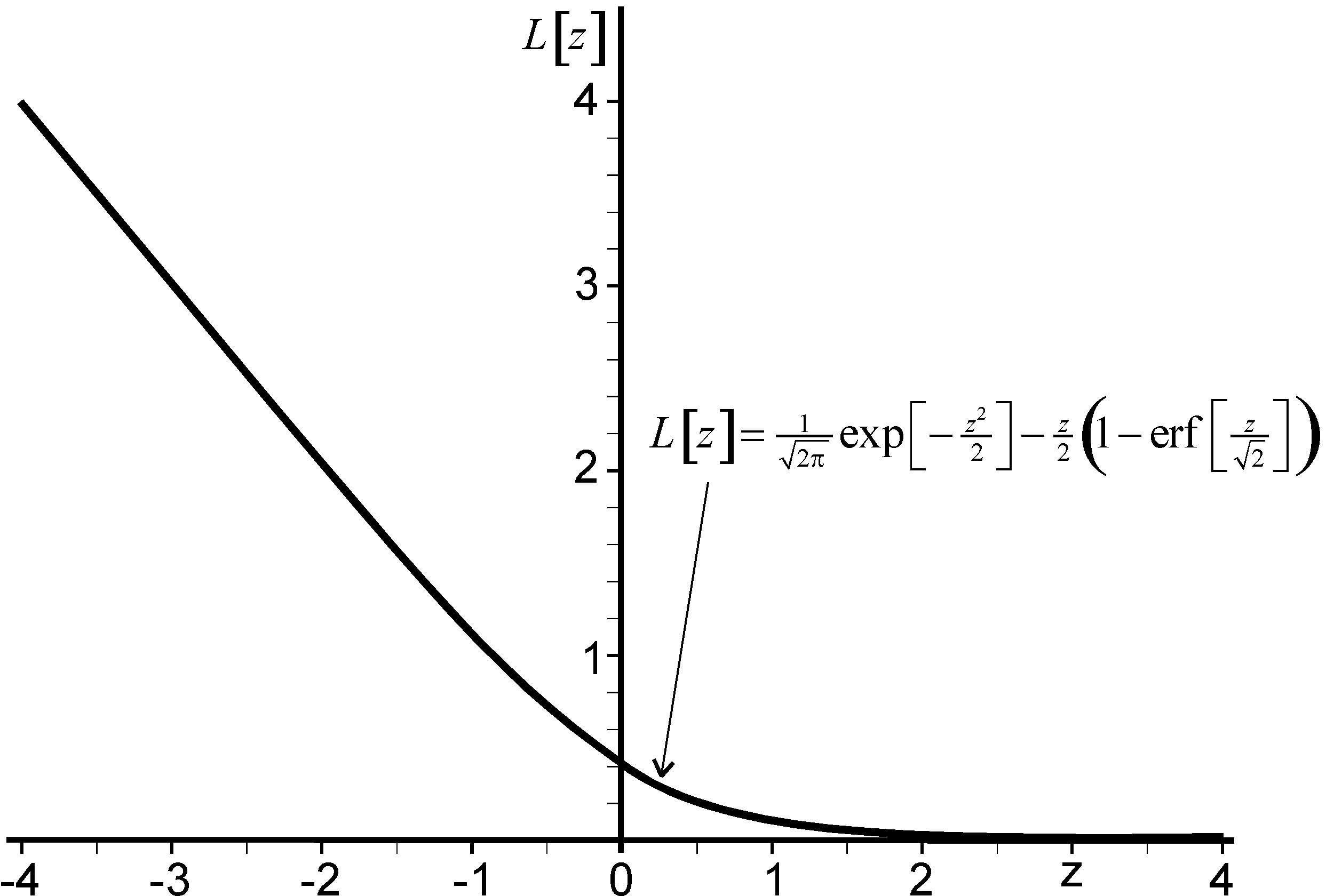
Figure D.3: The standard normal loss function
\(\forall z, L[z]>0\), and \(L[z]\) is a monotonically decreasing function in \(z\). Note that \(L'[z]=\Phi[z]-1\) which means that the loss function \(L[z]\) is decreasing and convex. The inverse loss function, \(L^{-1}[z]\) has no known solution. However it is easy to develop a User Defined Function in Microsoft Excel to calculate the inverse loss function. The Visual Basic code required is shown below. This can be saved as a “Microsoft Excel Add-In”. After such a procedure then “=InvLossFun(z)”, can be used within Microsoft Excel to calculate \(L^{-1}[z]\). A pre-made custom Excel Add-in is available here for download. To install this Add-in:
- Save the file onto your computer.
- Open Excel.
- Select Files/Options/Add-in/Manage Add-ins.
- Click ‘Go’.
- Browse to the folder where you saved the Add-in.
- Select the .xla file.
- Confirm the Operations Analysis Add-in is ticked in list of available Add-ins.
- When you have done this, the following functions should now be available in Excel:
Function InvLossFun(x As Double)
Dim u, l, z, p, b As Double
u = 6.1
l = -6.1
For g = 1 To 100000000
z = l + (( u - l) / 2)
p = (z / 2) * (1 - (2 * WorksheetFunction.NormDist(z, 0, 1, True) - 1)) + x
b = Exp( - (z ^ 2) / 2) / 2.506628274631
If p > b Then u = z Else l = z End If
If (u - l) < 0.000000000000001 Then g = 100000000 End If
Next g
InvLossFun = l + (( u - l) / 2)
End Function